Computing in Science Education; how to integrate Computing in Science Courses across Disciplines
University of Surrey, UK, November 28, 2017
Wouldn't it be cool if your mechanics students could reproduce results in a PRL?
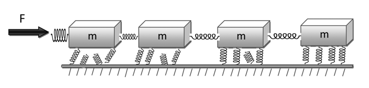
Grand challenge project in FYS-MEK1100 (Mechanics, University of Oslo), Second Semester: a friction model to be solved as coupled ODEs. And find problems with the article?

Unique opportunities
Computing competence represents a central element in scientific problem solving, from basic education and research to essentially almost all advanced problems in modern societies.
Computing competence enlarges the body of tools available to students and scientists beyond classical tools and allows for a more generic handling of problems. Focusing on algorithmic aspects results in deeper insights about scientific problems.
- Computing in basic physics courses allows us to bring important elements of scientific methods at a much earlier stage in our students' education.
- It gives the students skills and abilities that are asked for by society.
- It gives us as university teachers a unique opportunity to enhance students' insights about physics and how to solve scientific problems.
Computing competence
Computing means solving scientific problems using all possible tools, including symbolic computing, computers and numerical algorithms, and analytical paper and pencil solutions .
Computing is about developing an understanding of the scientific method by enhancing algorithmic thinking when solving problems.
On the part of students, this competence involves being able to:
- understand how algorithms are used to solve mathematical problems,
- derive, verify, and implement algorithms,
- understand what can go wrong with algorithms,
- use these algorithms to construct reproducible scientific outcomes and to engage in science in ethical ways, and
- think algorithmically for the purposes of gaining deeper insights about scientific problems.
Better understanding of the scientific method
All these elements are central for maturing and gaining a better understanding of the modern scientific process per se.
The power of the scientific method lies in identifying a given problem as a special case of an abstract class of problems, identifying general solution methods for this class of problems, and applying a general method to the specific problem (applying means, in the case of computing, calculations by pen and paper, symbolic computing, or numerical computing by ready-made and/or self-written software). This generic view on problems and methods is particularly important for understanding how to apply available, generic software to solve a particular problem.
Why should basic university education undergo a shift towards modern computing?
- Algorithms involving pen and paper are traditionally aimed at what we often refer to as continuous models.
- Application of computers calls for approximate discrete models.
- Much of the development of methods for continuous models are now being replaced by methods for discrete models in science and industry, simply because much larger classes of problems can be addressed with discrete models, often also by simpler and more generic methodologies.
However, verification of algorithms and understanding their limitations requires much of the classical knowledge about continuous models.
So, why should basic university education undergo a shift towards modern computing?
Why is computing competence important?
The impact of the computer on mathematics and science is tremendous: science and industry now rely on solving mathematical problems through computing.- Computing can increase the relevance in education by solving more realistic problems earlier.
- Computing through programming can be excellent training of creativity.
- Computing can enhance the understanding of abstractions and generalization.
- Computing can decrease the need for special tricks and tedious algebra, and shifts the focus to problem definition, visualization, and "what if" discussions.
Disasters attributable to poor management of code
Have you been paying attention in your numerical analysis or scientific computation courses? If not, it could be a costly mistake. Here are some real life examples of what can happen when numerical algorithms are not correctly applied.
- The Patriot Missile failure, in Dharan, Saudi Arabia, on February 25, 1991 which resulted in 28 deaths, is ultimately attributable to poor handling of rounding errors.
- The explosion of the Ariane 5 rocket just after lift-off on its maiden voyage off French Guiana, on June 4, 1996, was ultimately the consequence of a simple overflow.
- The sinking of the Sleipner A offshore platform in Gandsfjorden near Stavanger, Norway, on August 23, 1991, resulted in a loss of nearly one billion dollars. It was found to be the result of inaccurate finite element analysis.
- Add about Mars expedition
Modeling and computations as a way to enhance algorithminc thinking
Algorithmic thinking as a way to
- Enhance instruction based teaching
- Introduce Research based teaching from day one
- Trigger further insights in math and other disciplines
- Validation and verification of scientific results (the PRL example), with the possibility to emphasize ethical aspects as well. Version control is central.
- Good working practices from day one.
Can we catch many birds with one stone?
- How can we include and integrate an algorithmic (computational) perspective in our basic education?
- Can this enhance the students' understanding of mathematics and science?
- Can it strengthen research based teaching?
What is needed?
A compulsory programming course with a strong mathematical flavour. Should give a solid foundation in programming as a problem solving technique in mathematics. Programming is understanding! The line of thought when solving mathematical problems numerically enhances algorithmic thinking, and thereby the students' understanding of the scientific process.
Mathematics is at least as important as before, but should be supplemented with development, analysis, implementation, verification and validation of numerical methods. Science ethics and better understanding of the pedagogical process, almost for free!
Training in modeling and problem solving with numerical methods and visualisation, as well as traditional methods in Science courses, Physics, Chemistry, Biology, Geology, Engineering...
Implementation
- Support from governing bodies (high priorities at the College of Natural Science at UOslo and the Physics and Astronomy department of Michigan State University)
- Cooperation across departmental boundaries
- Willingness by individuals to give priority to teaching reform
Consensus driven approach.
Implementation in Oslo: The C(omputing in)S(cience)E(Education) project
- Coordinated use of computational exercises and numerical tools in most undergraduate courses.
- Help update the scientific staff's competence on computational aspects and give support (scientific, pedagogical and financial) to those who wish to revise their courses in a computational direction.
- Teachers get good summer students to aid in introducing computational exercises
- Develop courses and exercise modules with a computational perspective, both for students and teachers. New textbooks!!
- Basic idea: mixture of mathematics, computation, informatics and topics from the physical sciences.
Interesting outcome: higher focus on teaching and pedagogical issues!!
Example of bachelor program, Physics and Astronomy (astro path), University of Oslo
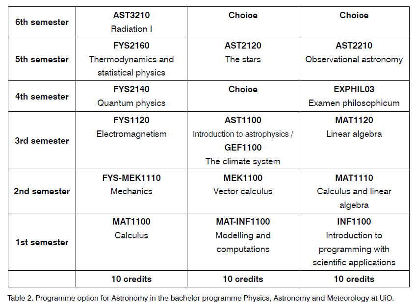
Example: Computations from day one
Three courses the first semester: MAT1100, MAT-INF1100 og INF1100.
- Definition of the derivative in MAT1100 (Calculus and analysis)
$$
f'(x)=\lim_{h \rightarrow 0}\frac{f(x+h)-f(x)}{h}.
$$
- Algorithms to compute the derivative in MAT-INF1100 (Mathematical modelling with computing)
$$
f'(x)= \frac{f(x+h)-f(x-h)}{2h}+O(h^2).
$$
- Implementation in Python in INF1100
def differentiate(f, x, h=1E-5):
     return (f(x+h) - f(x-h))/(2*h)
Example: Computations from day one
Combined with the possibility of symbolic calculations with Sympy, Python offers an environment where students and teachers alike can test many different aspects of mathematics and numerical mathematics, in addition to being able to verify and validate their codes. The following simple example shows how to extend the simple function for computing the numerical derivative with the possibility of obtaining the closed form or analytical expression
def differentiate(f, x, h=1E-5, symbolic=False):
    if symbolic:
        import sympy
        return sympy.lambdify([x], sympy.diff(f, x))
    else:
        return (f(x+h) - f(x-h))/(2*h)
Other Examples
- Definition of integration in MAT1100 (Calculus and analysis).
- The algorithm for computing the integral vha the Trapezoidal rule for an interval \( x \in [a,b] \)
$$
\int_a^b(f(x) dx \approx \frac{1}{2}\left [f(a)+2f(a+h)+\dots+2f(b-h)+f(b)\right]
$$
- Taught in MAT-INF1100 (Mathematical modelling)
- The algorithm is then implemented in INF1100 (programming course).
Typical implementation first semester of study
from math import exp, log, sin
def Trapez(a,b,f,n):
   h = (b-a)/float(n)
   s = 0
   x = a
   for i in range(1,n,1):
       x = x+h
       s = s+ f(x)
   s = 0.5*(f(a)+f(b)) +s
   return h*s

def f1(x):
    return exp(-x*x)*log(1+x*sin(x))

a = 1;  b = 3; n = 1000
result = Trapez(a,b,f1,n)
print(result)
Symbolic calculations and numerical calculations in one code
Python offers an extremely versatile programming environment, allowing for the inclusion of analytical studies in a numerical program. Here we show an example code with the trapezoidal rule using SymPy to evaluate an integral and compute the absolute error with respect to the numerically evaluated one of the integral \( \int_0^1 dx x^2 = 1/3 \):
Error analysis
The following extended version of the trapezoidal rule allows you to plot the relative error by comparing with the exact result. By increasing to \( 10^8 \) points one arrives at a region where numerical errors start to accumulate.
Integrating numerical mathematics with calculus
The last example shows the potential of combining numerical algorithms with symbolic calculations, allowing thereby students and teachers to
- Validate and verify their algorithms.
- Including concepts like unit testing, one has the possibility to test and validate several or all parts of the code.
- Validation and verification are then included naturally and one can develop a better attitude to what is meant with an ethically sound scientific approach.
- The above example allows the student to also test the mathematical error of the algorithm for the trapezoidal rule by changing the number of integration points. The students get trained from day one to think error analysis.
- With an Jupyter/Ipython notebook the students can keep exploring similar examples and turn them in as their own notebooks.
Additional benefits: A structured approach to solving problems
In this process we easily bake in
- How to structure a code in terms of functions
- How to make a module
- How to read input data flexibly from the command line
- How to create graphical/web user interfaces
- How to write unit tests (test functions or doctests)
- How to refactor code in terms of classes (instead of functions only)
- How to conduct and automate large-scale numerical experiments
- How to write scientific reports in various formats (LaTeX, HTML)
Additional benefits: A structure approach to solving problems
The conventions and techniques outlined here will save you a lot of time when you incrementally extend software over time from simpler to more complicated problems. In particular, you will benefit from many good habits:
- New code is added in a modular fashion to a library (modules)
- Programs are run through convenient user interfaces
- It takes one quick command to let all your code undergo heavy testing
- Tedious manual work with running programs is automated,
- Your scientific investigations are reproducible, scientific reports with top quality typesetting are produced both for paper and electronic devices.
Learning outcomes three first semesters
- Differential equations: Euler, modified Euler and Runge-Kutta methods (first semester)
- Numerical integration: Trapezoidal and Simpson's rule, multidimensional integrals (first semester)
- Random numbers, random walks, probability distributions and Monte Carlo integration (first semester)
- Linear Algebra and eigenvalue problems: Gaussian elimination, LU-decomposition, SVD, QR, Givens rotations and eigenvalues, Gauss-Seidel. (second and third semester)
- Root finding and interpolation etc. (all three first semesters)
- Processing of sound and images (first semester).
The students have to code several of these algorithms during the first three semesters.
Later courses
Later courses should build on this foundation as much as possible.
- In particular, the course should not be too basic! There should be progression in the use of mathematics, numerical methods and programming, as well as science.
- Computational platform: Python, fully object-oriented and allows for seamless integration of c++ and Fortran codes, as well as Matlab-like programming environment. Makes it easy to parallelize codes as well.
Coordination
- Teachers in other courses need therefore not use much time on numerical tools. Naturally included in other courses.
Challenges...
Standard objection: computations take away the attention from other central topics in 'my course'.
CSE incorporates computations from day one, and courses higher up do not need to spend time on computational topics (technicalities), but can focus on the interesting science applications. Coordination and synchronization across departments and courses. Increases collaboration on teaching and awareness of pedagical research.
- To help teachers: Developed pedagogical modules which can aid university teachers. Own course for teachers.
Examples of simple algorithms, initial value problems and proper scaling of equations
- Ordinary differential equations (ODE): RLC circuit
- ODE: Classical pendulum
- ODE: Solar system
- and many more cases
Can use essentially the same algorithms to solve these problems, either some simple modified Euler algorithms or some Runge-Kutta class of algorithms or perhaps the so-called Verlet class of algorithms. Algorithms students use in one course can be reused in other courses.
Mechanics and electromagnetism, initial value problems
Classical pendulum with damping and external force as it could appear in a mechanics course (PHY 321)
$$
ml\frac{d^2\theta}{dt^2}+\nu\frac{d\theta}{dt} +mgsin(\theta)=Acos(\omega t).
$$
Easy to solve numerically and then visualize the solution.
Almost the same equation for an RLC circuit in the electromagnetism course (PHY 482)
$$
L\frac{d^2Q}{dt^2}+\frac{Q}{C}+R\frac{dQ}{dt}=Acos(\omega t).
$$
Mechanics and electromagnetism, initial value problems and now proper scaling
Classical pendulum equations with damping and external force
$$
\frac{d\theta}{d\hat{t}} =\hat{v},
$$
and
$$
\frac{d\hat{v}}{d\hat{t}} =Acos(\hat{\omega} \hat{t})-\hat{v}\xi-\sin(\theta),
$$
with \( \omega_0=\sqrt{g/l} \), \( \hat{t}=\omega_0 t \) and \( \xi = mg/\omega_0\nu \).
The RLC circuit
$$
\frac{dQ}{d\hat{t}} =\hat{I},
$$
and
$$
\frac{d\hat{I}}{d\hat{t}} =Acos(\hat{\omega} \hat{t})-\hat{I}\xi-Q,
$$
with \( \omega_0=1/\sqrt{LC} \), \( \hat{t}=\omega_0 t \) and \( \xi = CR\omega_0 \).
The equations are essentially the same. Great potential for abstraction.
Other examples of simple algorithms that can be reused in many courses, two-point boundary value problems and scaling
These physics examples can all be studied using almost the same types of algorithms, simple eigenvalue solvers and Gaussian elimination with the same starting matrix!
- A buckling beam and Toeplitz matrices (mechanics and mathematical methods), eigenvalue problems
- A particle in an infinite potential well, quantum eigenvalue problems
- A particle (or two) in a general quantum well, quantum eigenvalue problems
- Poisson's equation in one dim, linear algebra (electromagnetism)
- The diffusion equation in one dimension (Statistical Physics), linear algebra
- and many other cases
A buckling beam, or a quantum mechanical particle in an infinite well
This is a two-point boundary value problem
$$
R \frac{d^2 u(x)}{dx^2} = -F u(x),
$$
where \( u(x) \) is the vertical displacement, \( R \) is a material specific constant, \( F \) the force and \( x \in [0,L] \) with \( u(0)=u(L)=0 \).
Scale equations with \( x = \rho L \) and \( \rho \in [0,1] \) and get (note that we change from \( u(x) \) to \( v(\rho) \))
$$
\frac{d^2 v(\rho)}{dx^2} +K v(\rho)=0,
$$
a standard eigenvalue problem with \( K= FL^2/R \).
If you replace \( R=-\hbar^2/2m \) and \( -F=\lambda \), we have the quantum mechanical variant for a particle moving in a well with infinite walls at the endpoints.
Discretize and get the same type of problem
Discretize the second derivative and the rhs
$$
-\frac{v_{i+1} -2v_i +v_{i-i}}{h^2}=\lambda v_i,
$$
with \( i=1,2,\dots, n \). We need to add to this system the two boundary conditions \( v(0) =v_0 \) and \( v(1) = v_{n+1} \).
The so-called Toeplitz matrix (special case from the discretized second derivative)
$$
\mathbf{A} = \frac{1}{h^2}\begin{bmatrix}
2 & -1 & & & & \\
-1 & 2 & -1 & & & \\
& -1 & 2 & -1 & & \\
& \dots & \dots &\dots &\dots & \dots \\
& & &-1 &2& -1 \\
& & & &-1 & 2 \\
\end{bmatrix}
$$
with the corresponding vectors \( \mathbf{v} = (v_1, v_2, \dots,v_n)^T \) allows us to rewrite the differential equation
including the boundary conditions as a standard eigenvalue problem
$$
\mathbf{A}\mathbf{v} = \lambda\mathbf{v}.
$$
The Toeplitz matrix has analytical eigenpairs!! Adding a potential along the diagonals allows us to reuse this problem for many types of physics cases.
Adding complexity, hydrogen-like atoms or other one-particle potentials
We are first interested in the solution of the radial part of Schroedinger's equation for one electron. This equation reads
$$
-\frac{\hbar^2}{2 m} \left ( \frac{1}{r^2} \frac{d}{dr} r^2
\frac{d}{dr} - \frac{l (l + 1)}{r^2} \right )R(r)
+ V(r) R(r) = E R(r).
$$
Suppose in our case \( V(r) \) is the harmonic oscillator potential \( (1/2)kr^2 \) with
\( k=m\omega^2 \) and \( E \) is
the energy of the harmonic oscillator in three dimensions.
The oscillator frequency is \( \omega \) and the energies are
$$
E_{nl}= \hbar \omega \left(2n+l+\frac{3}{2}\right),
$$
with \( n=0,1,2,\dots \) and \( l=0,1,2,\dots \).
Scaling the equations
We introduce a dimensionless variable \( \rho = (1/\alpha) r \) where \( \alpha \) is a constant with dimension length and get
$$
-\frac{\hbar^2}{2 m \alpha^2} \frac{d^2}{d\rho^2} v(\rho)
+ \left ( V(\rho) + \frac{l (l + 1)}{\rho^2}
\frac{\hbar^2}{2 m\alpha^2} \right ) v(\rho) = E v(\rho) .
$$
Let us choose \( l=0 \).
Inserting \( V(\rho) = (1/2) k \alpha^2\rho^2 \) we end up with
$$
-\frac{\hbar^2}{2 m \alpha^2} \frac{d^2}{d\rho^2} v(\rho)
+ \frac{k}{2} \alpha^2\rho^2v(\rho) = E v(\rho) .
$$
We multiply thereafter with \( 2m\alpha^2/\hbar^2 \) on both sides and obtain
$$
-\frac{d^2}{d\rho^2} v(\rho)
+ \frac{mk}{\hbar^2} \alpha^4\rho^2v(\rho) = \frac{2m\alpha^2}{\hbar^2}E v(\rho) .
$$
A natural length scale comes out automagically when scaling
We have thus
$$
-\frac{d^2}{d\rho^2} v(\rho)
+ \frac{mk}{\hbar^2} \alpha^4\rho^2v(\rho) = \frac{2m\alpha^2}{\hbar^2}E v(\rho) .
$$
The constant \( \alpha \) can now be fixed
so that
$$
\frac{mk}{\hbar^2} \alpha^4 = 1,
$$
and it defines a natural length scale (like the Bohr radius does)
$$
\alpha = \left(\frac{\hbar^2}{mk}\right)^{1/4}.
$$
Defining
$$
\lambda = \frac{2m\alpha^2}{\hbar^2}E,
$$
we can rewrite Schroedinger's equation as
$$
-\frac{d^2}{d\rho^2} v(\rho) + \rho^2v(\rho) = \lambda v(\rho) .
$$
This is similar to the equation for a buckling beam except for the potential term.
In three dimensions
the eigenvalues for \( l=0 \) are
\( \lambda_0=1.5,\lambda_1=3.5,\lambda_2=5.5,\dots . \)
Discretizing
Define first the diagonal matrix element
$$
d_i=\frac{2}{h^2}+V_i,
$$
and the non-diagonal matrix element
$$
e_i=-\frac{1}{h^2}.
$$
In this case the non-diagonal matrix elements are given by a mere constant. All non-diagonal matrix elements are equal.
With these definitions the Schroedinger equation takes the following form
$$
d_iu_i+e_{i-1}v_{i-1}+e_{i+1}v_{i+1} = \lambda v_i,
$$
where \( v_i \) is unknown. We can write the
latter equation as a matrix eigenvalue problem
$$
\begin{equation}
\begin{bmatrix} d_1 & e_1 & 0 & 0 & \dots &0 & 0 \\
e_1 & d_2 & e_2 & 0 & \dots &0 &0 \\
0 & e_2 & d_3 & e_3 &0 &\dots & 0\\
\dots & \dots & \dots & \dots &\dots &\dots & \dots\\
0 & \dots & \dots & \dots &\dots &d_{n_{\mathrm{step}}-2} & e_{n_{\mathrm{step}}-1}\\
0 & \dots & \dots & \dots &\dots &e_{n_{\mathrm{step}}-1} & d_{n_{\mathrm{step}}-1}
\end{bmatrix} \begin{bmatrix} v_{1} \\
v_{2} \\
\dots\\ \dots\\ \dots\\
v_{n_{\mathrm{step}}-1}
\end{bmatrix}=\lambda \begin{bmatrix}{c} v_{1} \\
v_{2} \\
\dots\\ \dots\\ \dots\\
v_{n_{\mathrm{step}}-1}
\end{bmatrix}
\tag{1}
\end{equation}
$$
or if we wish to be more detailed, we can write the tridiagonal matrix as
$$
\begin{equation}
\left( \begin{array}{ccccccc} \frac{2}{h^2}+V_1 & -\frac{1}{h^2} & 0 & 0 & \dots &0 & 0 \\
-\frac{1}{h^2} & \frac{2}{h^2}+V_2 & -\frac{1}{h^2} & 0 & \dots &0 &0 \\
0 & -\frac{1}{h^2} & \frac{2}{h^2}+V_3 & -\frac{1}{h^2} &0 &\dots & 0\\
\dots & \dots & \dots & \dots &\dots &\dots & \dots\\
0 & \dots & \dots & \dots &\dots &\frac{2}{h^2}+V_{n_{\mathrm{step}}-2} & -\frac{1}{h^2}\\
0 & \dots & \dots & \dots &\dots &-\frac{1}{h^2} & \frac{2}{h^2}+V_{n_{\mathrm{step}}-1}
\end{array} \right)
\tag{2}
\end{equation}
$$
The Python code
The code sets up the Hamiltonian matrix by defining the minimun and maximum values of \( r \) with a maximum value of integration points. It plots the eigenfunctions of the three lowest eigenstates.
The power of numerical methods
The last example shows the potential of combining numerical algorithms with analytical results (or eventually symbolic calculations), allowing thereby students and teachers to
- make abstraction and explore other physics cases easily where no analytical solutions are known
- Validate and verify their algorithms.
- Including concepts like unit testing, one has the possibility to test and validate several or all parts of the code.
- Validation and verification are then included naturally and one can develop a better attitude to what is meant with an ethically sound scientific approach.
- The above example allows the student to also test the mathematical error of the algorithm for the eigenvalue solver by changing the number of integration points. The students get trained from day one to think error analysis.
- The algorithm can be tailored to any kind of one-particle problem used in quantum mechanics or eigenvalue problems
- A simple rewrite allows for reuse in linear algebra problems for solution of say Poisson's equation in electromagnetism, or the diffusion equation in one dimension.
- With an ipython notebook students can keep exploring similar examples and turn them in as their own notebooks.
Which aspects are important for a successful introduction of CSE?
- Early introduction, programming course at beginning of studies linked with math courses and science and engineering courses.
- Crucial to learn proper programming at the beginning.
- Good TAs
- Choice of software.
- Textbooks and modularization of topics, ask for details
- Resources and expenses.
- Tailor to specific disciplines.
- Organizational matters.
- With a local physics education group one can do much more!! At MSU we have a very strong Physics Education Research group headed by Danny Caballero and Washti Sawtelle
Summary
- Make our research visible in early undergraduate courses, enhance research based teaching
- Possibility to focus more on understanding and increased insight.
- Impetus for broad cooperation in teaching. Broad focus on university pedagogical topics.
- Strengthening of instruction based teaching (expensive and time-consuming).
- Give our candidates a broader and more up-to-date education with a problem-based orientation, often requested by potential employers.
- And perhaps the most important issue: does this enhance the student's insight in the Sciences?
We invite you to visit (online and/or in real life) our new center on Computing in Science Education
More links
- Python and our first programming course, first semester course. Excellent new textbook by Hans Petter Langtangen, click here for the textbook or the online version
- Mathematical modelling course, first semester course. Textbook by Knut Morken to be published by Springer.
- Mechanics, second semester course. New textbook by Anders Malthe-Sorenssen, published by Springer, Undergraduate Lecture Notes in Physics
- Computational Physics I, fifth semester course. Textbook to be published by IOP, with online version
- Book on waves and motion, Statistical Physics and Quantum physics to come, stay tuned!!
What about life science/biology? Overarching questions
There is new demand for more
- quantitative methods & reasoning
- understanding data and phenomena via models
- creating in silico virtual labs
How to integrate such computing-based activities in the undergraduate programs when the students are not interested in mathematics, physics, and programming?
How to teach computing in biology?
Do we need to still follow the tradition and teach mathematics, physics, computations, chemistry, etc. in separate discipline-specific courses?
- Uninteresting to first study tools when you want to study biology
- Little understanding of what the tools are good for
- Minor utilization of tools later in biology
It's time for new thinking
- Just-in-time teaching: teach tools when needed
- Teach tools in the context of biology
- Emphasize development of intuition and understanding
- Base learning of the students' own explorations in biology projects
- Integrate lab work with computing tools
The pedagogical framework
- Method: case-based learning
- Coherent problem solving in biology by integrating mathematics, programming, physics/chemistry, ...
- Starting point: data from lab or field experiments
- Visualize data
- Derive computational models directly from mathematical/intuitive reasoning
- Program model(s), fit parameters, compare with data
- Develop intuition and understanding based on
- the principles behind the model
- exploration of the model ("what if")
- prediction of new experiments
Example 1: ecoli lab experiment
Observations of no of bacteria vs time in seconds, stored in Excel and written to a CVS file:
0,100
600,140
1200,250
1800,360
2400,480
3000,820
3600,1300
4200,1700
4800,2900
5400,3900
6000,7000
Visualize data
- Meet a text editor and a terminal window
- Very basic Unix
First program:
t = [0, 600, 1200, 1800, 2400, 3000, 3600,
     4200, 4800, 5400, 6000]
N = [100, 140, 250, 360, 480, 820, 1300, 1700, 2900, 3900, 7000]
import matplotlib.pyplot as plt
plt.plot(t, N, 'ro')
plt.xlabel('t [s]')
plt.ylabel('N')
plt.show()
Concepts must be introduced implicitly in a structured way
- Always identify new concepts
- Train new concepts in simplified ("trivial") problems
Concepts in the previous example:
- Lists or arrays of numbers
- Plotting commands
- Curve = function of time
The concept of a continuous function \( N(t) \) is not necessary, just straight lines between discrete points on a curve.
Read data from file
import numpy as np
data = np.loadtxt('src/ecoli.csv', delimiter=',')
print data  # look at the format
t = data[:,0]
N = data[:,1]
import matplotlib.pyplot as plt
plt.plot(t, N, 'ro')
plt.xlabel('t [s]')
plt.ylabel('N')
plt.show()
The population grows faster and faster. Why? Is there an underlying (general) mechanism?
Lab journal
Use IPython notebook as lab journal.
How can we reason about the process?
- Cells divide after \( T \) seconds on average (one generation)
- \( 2N \) celles divide into twice as many new cells \( \Delta N \) in a time interval \( \Delta t \) as \( N \) cells would: \( \Delta N \propto N \)
- \( N \) cells result in twice as many new individuals \( \Delta N \) in time \( 2\Delta t \) as in time \( \Delta t \): \( \Delta N \propto\Delta t \)
- Same proportionality wrt death (repeat reasoning)
- Proposed model: \( \Delta N = b\Delta t N - d\Delta tN \) for some unknown constants \( b \) (births) and \( d \) (deaths)
- Describe evolution in discrete time: \( t_n=n\Delta t \)
- Program-friendly notation: \( N \) at \( t_n \) is \( N^n \)
- Math model: \( N^{n+1} = N^n + r\Delta t\, N \) (with \( \ r=b-d \))
- Program model:
N[n+1] = N[n] + r*dt*N[n]
The first simple program
Let us solve the difference equation in as simple way as possible, just to train some programming: \( r=1.5 \), \( N^0=1 \), \( \Delta t=0.5 \)
import numpy as np

t = np.linspace(0, 10, 21)  # 20 intervals in [0, 10]
dt = t[1] - t[0]
N = np.zeros(t.size)

N[0] = 1
r = 0.5

for n in range(0, N.size-1, 1):
    N[n+1] = N[n] + r*dt*N[n]
    print 'N[%d]=%.1f' % (n+1, N[n+1])
The output
N[1]=1.2
N[2]=1.6
N[3]=2.0
N[4]=2.4
N[5]=3.1
N[6]=3.8
N[7]=4.8
N[8]=6.0
N[9]=7.5
N[10]=9.3
N[11]=11.6
N[12]=14.6
N[13]=18.2
N[14]=22.7
N[15]=28.4
N[16]=35.5
N[17]=44.4
N[18]=55.5
N[19]=69.4
N[20]=86.7
Parameter estimation
- We do not know \( r \)
- How can we estimate \( r \) from data?
We can use the difference equation with the experimental data
$$ N^{n+1} = N^n + r\Delta t N^n$$
Say \( N^{n+1} \) and \( N^n \) are known from data, solve wrt \( r \):
$$ r = \frac{N^{n+1}-N^n}{N^n\Delta t} $$
Use experimental data in the fraction, say \( t_1=600 \), \( t_2=1200 \), \( N^1=140 \), \( N^2=250 \): \( r=0.0013 \).
Can do a nonlinear least squares parameter fit, but that is too advanced at this stage.
A program relevant for the biological problem
import numpy as np

# Estimate r
data = np.loadtxt('ecoli.csv', delimiter=',')
t_e = data[:,0]
N_e = data[:,1]
i = 2  # Data point (i,i+1) used to estimate r
r = (N_e[i+1] - N_e[i])/(N_e[i]*(t_e[i+1] - t_e[i]))
print 'Estimated r=%.5f' % r
# Can experiment with r values and see if the model can
# match the data better

T = 1200     # cell can divide after T sec
t_max = 5*T  # 5 generations in experiment
t = np.linspace(0, t_max, 1000)
dt = t[1] - t[0]
N = np.zeros(t.size)

N[0] = 100
for n in range(0, len(t)-1, 1):
    N[n+1] = N[n] + r*dt*N[n]

import matplotlib.pyplot as plt
plt.plot(t, N, 'r-', t_e, N_e, 'bo')
plt.xlabel('time [s]');  plt.ylabel('N')
plt.legend(['model', 'experiment'], loc='upper left')
plt.show()
Change r in the program and play around to make a better fit!
Discuss the nature of such a model
- Write up all the biological factors that influence the population size of bacteria
- Understand that all such effects are merged into one parameter \( r \)
- Understand that the reasoning must be the same whether we
have bacteria, animals or humans - this is a generic model!
(even the interest rate in a bank follows the same model)
Discuss the limitations of such a model
- How many bacteria in the lab after one month?
- Growth is restricted by environmental resources!
- Fix the model (logistic growth)
- Is the logistic model appropriate for a lab experiment?
- Find data to support the logistic model
(it's a very simple model)
The pedagogical template (to be iterated!)
- Start with a real biological problem
- Be careful with too many new concepts
- Workflow:
- data
- visualization
- patterns
- modeling (discrete)
- programming
- testing
- parameter estimation (difficult)
- validation
- prediction
- Make many small exercises that train the new concepts
- Repeat the case in a way that makes a complete understanding