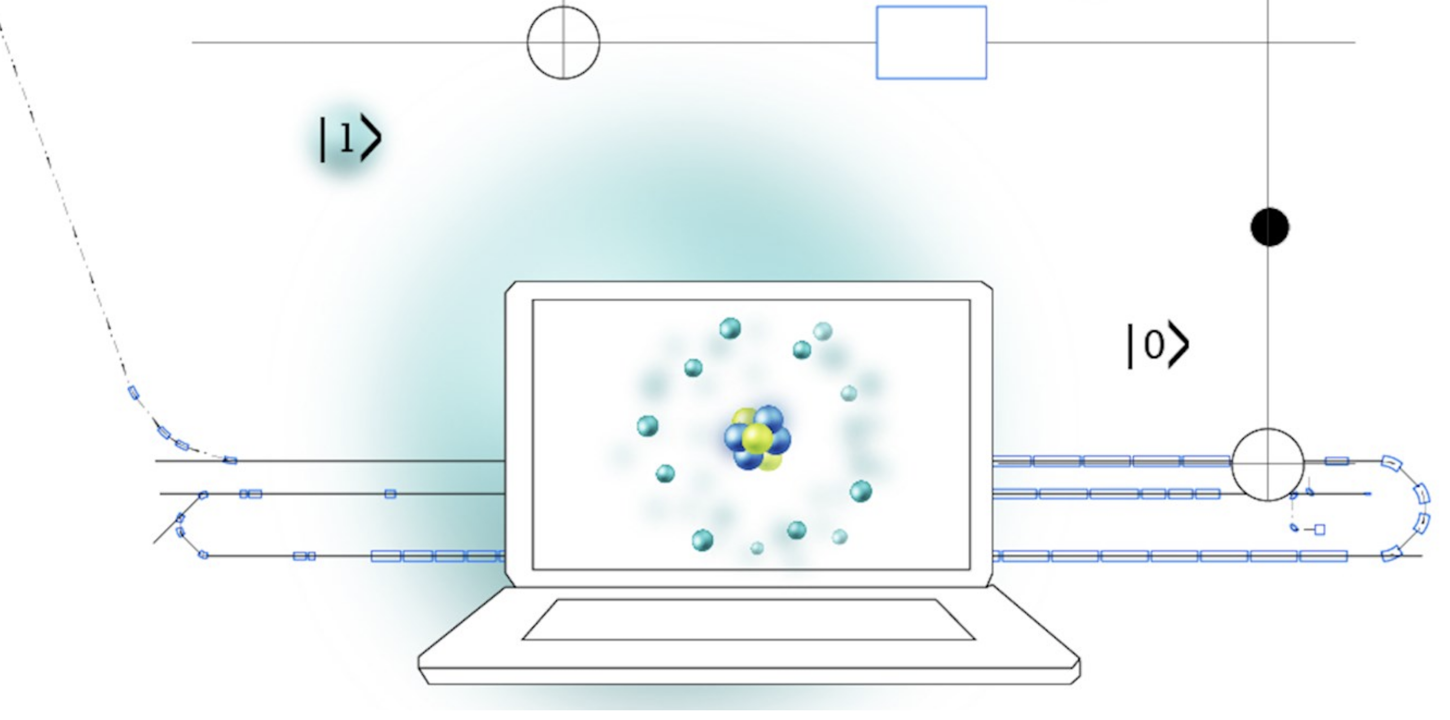
Machine Learning meets Quantum Physics
XAI: Explaining what goes on inside DNN/AI, December 8, 2020, Oslo, Norway
What is this talk about?
The main aim is to give you a short and pedestrian introduction to how we can use Machine Learning methods to solve quantum mechanical many-body problems and how we can use such techniques. And why this could be of interest.
The hope is that after this talk you have gotten the basic ideas to get you started. Peeping into https://github.com/mhjensenseminars/MachineLearningTalk, you'll find a Jupyter notebook, slides, codes etc that will allow you to reproduce the simulations discussed here, and perhaps run your own very first calculations.
Quantum Computing and Machine Learning
Quantum Computing and Machine Learning are two of the most promising approaches for studying complex physical systems where several length and energy scales are involved. Traditional many-particle methods, either quantum mechanical or classical ones, face huge dimensionality problems when applied to studies of systems with many interacting particles.
More material on Machine Learning and Quantum Mechanics
More in depth notebooks and lecture notes are at
- Making a professional Monte Carlo code for quantum mechanical simulations https://github.com/CompPhysics/ComputationalPhysics2/blob/gh-pages/doc/pub/notebook1/ipynb/notebook1.ipynb
- From Variational Monte Carlo to Boltzmann Machines https://github.com/CompPhysics/ComputationalPhysics2/blob/gh-pages/doc/pub/notebook2/ipynb/notebook2.ipynb
- Nuclear Talent course on Machine Learning in Nuclear Experiment and Theory, June 22 - July 3, 2020
Feel free to try them out and please don't hesitate to ask if something is unclear.
Why? Basic motivation
How can we avoid the dimensionality curse? Many possibilities
- smarter basis functions
- resummation of specific correlations
- stochastic sampling of high-lying states (stochastic FCI, CC and SRG/IMSRG)
- many more
Machine Learning and Quantum Computing hold also great promise in tackling the ever increasing dimensionalities. Here we will focus on Machine Learning, with some links to recent research to quantum machine learning.
Overview
- Short intro to Machine Learning
- Variational Monte Carlo (Markov Chain Monte Carlo, \( \mathrm{MC}^2 \)) and many-body problems, solving quantum mechanical problems in a stochastic way. It will serve as our motivation for switching to Machine Learning.
- From Variational Monte Carlo to Boltzmann Machines and Deep Learning
- And then to Quantum Computing and Machine Learning
Machine Learning and AI and Physics
Artificial intelligence-based techniques, particularly in machine learning and optimization, are increasingly being used in many areas of experimental and theoretical physics to facilitate discovery, accelerate data analysis and modeling efforts, and bridge different physical and temporal scales in numerical models.
These techniques are proving to be powerful tools for advancing our understanding; however, they are not without significant challenges. The theoretical foundations of many tools, such as deep learning, are poorly understood, resulting in the use of techniques whose behavior (and misbehavior) is difficult to predict and understand. Similarly, physicists typically use general AI techniques that are not tailored to the needs of the experimental and theoretical work being done. Thus, many opportunities exist for major advances both in physical discovery using AI and in the theory of AI. Furthermore, there are tremendous opportunities for these fields to inform each other, for example, in creating machine learning- based methods that must obey certain constraints by design, such as the conservation of mass, momentum and energy.
A new world
Machine learning is an extremely rich field, in spite of its young age. The increases we have seen during the last three decades in computational capabilities have been followed by developments of methods and techniques for analyzing and handling large date sets, relying heavily on statistics, computer science and mathematics. The field is rather new and developing rapidly.
Popular software packages written in Python for ML are
and more. These are all freely available at their respective GitHub sites. They encompass communities of developers in the thousands or more. And the number of code developers and contributors keeps increasing.
Lots of room for creativity
Not all the algorithms and methods can be given a rigorous mathematical justification, opening up thereby for experimenting and trial and error and thereby exciting new developments.
A solid command of linear algebra, multivariate theory, probability theory, statistical data analysis, optimization algorithms, understanding errors and Monte Carlo methods is important in order to understand many of the various algorithms and methods.
Job market, a personal statement: A familiarity with ML is almost becoming a prerequisite for many of the most exciting employment opportunities. And add quantum computing and there you are!
Types of Machine Learning
The approaches to machine learning are many, but are often split into two main categories. In supervised learning we know the answer to a problem, and let the computer deduce the logic behind it. On the other hand, unsupervised learning is a method for finding patterns and relationship in data sets without any prior knowledge of the system. Some authours also operate with a third category, namely reinforcement learning. This is a paradigm of learning inspired by behavioural psychology, where learning is achieved by trial-and-error, solely from rewards and punishment.
Another way to categorize machine learning tasks is to consider the desired output of a system. Some of the most common tasks are:
- Classification: Outputs are divided into two or more classes. The goal is to produce a model that assigns inputs into one of these classes. An example is to identify digits based on pictures of hand-written ones. Classification is typically supervised learning.
- Regression: Finding a functional relationship between an input data set and a reference data set. The goal is to construct a function that maps input data to continuous output values.
- Clustering: Data are divided into groups with certain common traits, without knowing the different groups beforehand. It is thus a form of unsupervised learning.
A simple perspective on the interface between ML and Physics

ML in Physics, Examples
The large amount of degrees of freedom pertain to both theory and experiment in physics. With increasingly complicated experiments that produce large amounts data, automated classification of events becomes increasingly important. Here, deep learning methods offer a plethora of interesting research avenues.
- Reconstruction of particle trajectories or classification of events are typical examples where ML methods are being used. However, since these data can often be extremely noisy, the precision necessary for discovery in physics requires algorithmic improvements. Research along such directions, interfacing nuclear physics with AI/ML is expected to play a significant role in physics discoveries related to new facilities. The treatment of corrupted data in imaging and image processing is also a relevant topic.
- Design of detectors represents an important area of applications for ML/AI methods in subnuclear physics.
- Many of the above classification problems have also have direct application in theoretical physics.
More examples
- An important application of AI/L methods is to improve the estimation of bias or uncertainty due to the introduction of or lack of physical constraints in various theoretical models.
- In theory, we expect to use AI/ML algorithms and methods to improve our knowledged about correlations of physical model parameters in data for quantum many-body systems. Deep learning methods like Boltzmann machines and various types of Recurrent Neural networks show great promise in circumventing the exploding dimensionalities encountered in quantum mechanical many-body studies.
- Merging a frequentist approach (the standard path in ML theory) with a Bayesian approach, has the potential to infer better probabilitity distributions and error estimates. As an example, methods for fast Monte-Carlo- based Bayesian computation of nuclear density functionals show great promise in providing a better understanding
- Machine Learning and Quantum Computing is a very interesting avenue to explore and a hot research topic.
From Classical Computations to Quantum Data and Quantum Machine Learning

Selected References in Machine Learning
- An excellent reference, Mehta et al. and Physics Reports (2019).
- Machine Learning and the Physical Sciences by Carleo et al
- Ab initio solution of the many-electron Schrödinger equation with deep neural networks by Pfau et al..
- Machine Learning and the Deuteron by Kebble and Rios
- Variational Monte Carlo calculations of \( A\le 4 \) nuclei with an artificial neural-network correlator ansatz by Adams et al.
- Unsupervised Learning for Identifying Events in Active Target Experiments by Solli et al.
- Report from the A.I. For Nuclear Physics Workshop by Bedaque et al.
References on Quantum Machine Learning
- Amin et al., Quantum Boltzmann Machines, Physical Review X 8, (2018)
- Zoufal et al., Variational Quantum Boltzmann Machines, ArXiv.2006.0004
- Maria Schuld and Francesco Petruccione, Supervised Machine Learning with Quantum Computers, Springer, 2018
- Yuan et al., Theory of Variational Quantum Simulations, ArXiv.1812.08767
Highly recommended: Sofia Vallecorsa's lecture on Quantum Machine Learning and slides.
See also interview with Maria Schuld.
Applications of Quantum Machine Learning
- Quantum Support Vector Machines for Higgs boson classification
- Quantum Graph Neural Networks for particle trajectory reconstruction/pattern recognition
- Quantum Generative Adversarial Networks for detector simulation
- Quantum Boltzman Machines for reinforcement learning
See Sofia Vallecorsa's lecture on Quantum Machine Learning and CERN related activities and slides.
What are the Machine Learning calculations here based on?
This work is inspired by the idea of representing the wave function with a restricted Boltzmann machine (RBM), presented recently by G. Carleo and M. Troyer, Science 355, Issue 6325, pp. 602-606 (2017). They named such a wave function/network a neural network quantum state (NQS). In their article they apply it to the quantum mechanical spin lattice systems of the Ising model and Heisenberg model, with encouraging results. See also the recent work by Adams et al..
Thanks to Daniel Bazin (MSU), Jane Kim (MSU), Julie Butler (MSU), Sean Liddick (MSU), Michelle Kuchera (Davidson College), Vilde Flugsrud (UiO), Even Nordhagen (UiO), Bendik Samseth (UiO) and Robert Solli (UiO) for many discussions and interpretations.
A Frequentist approach to data analysis
When you hear phrases like predictions and estimations and correlations and causations, what do you think of? May be you think of the difference between classifying new data points and generating new data points. Or perhaps you consider that correlations represent some kind of symmetric statements like if \( A \) is correlated with \( B \), then \( B \) is correlated with \( A \). Causation on the other hand is directional, that is if \( A \) causes \( B \), \( B \) does not necessarily cause \( A \).
These concepts are in some sense the difference between machine learning and statistics. In machine learning and prediction based tasks, we are often interested in developing algorithms that are capable of learning patterns from given data in an automated fashion, and then using these learned patterns to make predictions or assessments of newly given data. In many cases, our primary concern is the quality of the predictions or assessments, and we are less concerned about the underlying patterns that were learned in order to make these predictions.
In machine learning we normally use a so-called frequentist approach, where the aim is to make predictions and find correlations. We focus less on for example extracting a probability distribution function (PDF). The PDF can be used in turn to make estimations and find causations such as given \( A \) what is the likelihood of finding \( B \).
What are the basic ingredients?
Almost every problem in ML and data science starts with the same ingredients:
- The dataset \( \mathbf{x} \) (could be some observable quantity of the system we are studying)
- A model which is a function of a set of parameters \( \mathbf{\alpha} \) that relates to the dataset, say a likelihood function \( p(\mathbf{x}\vert \mathbf{\alpha}) \) or just a simple model \( f(\mathbf{\alpha}) \)
- A so-called loss/cost/risk function \( \mathcal{C} (\mathbf{x}, f(\mathbf{\alpha})) \) which allows us to decide how well our model represents the dataset.
We seek to minimize the function \( \mathcal{C} (\mathbf{x}, f(\mathbf{\alpha})) \) by finding the parameter values which minimize \( \mathcal{C} \). This leads to various minimization algorithms. It may surprise many, but at the heart of all machine learning algortihms there is an optimization problem.
Artificial neurons
The field of artificial neural networks has a long history of development, and is closely connected with the advancement of computer science and computers in general. A model of artificial neurons was first developed by McCulloch and Pitts in 1943 to study signal processing in the brain and has later been refined by others. The general idea is to mimic neural networks in the human brain, which is composed of billions of neurons that communicate with each other by sending electrical signals. Each neuron accumulates its incoming signals, which must exceed an activation threshold to yield an output. If the threshold is not overcome, the neuron remains inactive, i.e. has zero output.
This behaviour has inspired a simple mathematical model for an artificial neuron.
$$
y = f\left(\sum_{i=1}^n w_ix_i\right) = f(u)
$$
Here, the output \( y \) of the neuron is the value of its activation function, which have as input
a weighted sum of signals \( x_i, \dots ,x_n \) received by \( n \) other neurons.
A simple perceptron model

Neural network types
An artificial neural network (NN), is a computational model that consists of layers of connected neurons, or nodes. It is supposed to mimic a biological nervous system by letting each neuron interact with other neurons by sending signals in the form of mathematical functions between layers. A wide variety of different NNs have been developed, but most of them consist of an input layer, an output layer and eventual layers in-between, called hidden layers. All layers can contain an arbitrary number of nodes, and each connection between two nodes is associated with a weight variable.

Hybrid Quantum Computing and Machine Learning Network

The first system: electrons in a harmonic oscillator trap in two dimensions
The Hamiltonian of the quantum dot is given by
$$ \hat{H} = \hat{H}_0 + \hat{V},
$$
where \( \hat{H}_0 \) is the many-body HO Hamiltonian, and \( \hat{V} \) is the
inter-electron Coulomb interactions. In dimensionless units,
$$ \hat{V}= \sum_{i < j}^N \frac{1}{r_{ij}},
$$
with \( r_{ij}=\sqrt{\mathbf{r}_i^2 - \mathbf{r}_j^2} \).
This leads to the separable Hamiltonian, with the relative motion part given by (\( r_{ij}=r \))
$$
\hat{H}_r=-\nabla^2_r + \frac{1}{4}\omega^2r^2+ \frac{1}{r},
$$
plus a standard Harmonic Oscillator problem for the center-of-mass motion.
This system has analytical solutions in two and three dimensions (M. Taut 1993 and 1994).
Quantum Monte Carlo Motivation
Given a hamiltonian \( H \) and a trial wave function \( \Psi_T \), the variational principle states that the expectation value of \( \langle H \rangle \), defined through
$$
\langle E \rangle =
\frac{\int d\boldsymbol{R}\Psi^{\ast}_T(\boldsymbol{R})H(\boldsymbol{R})\Psi_T(\boldsymbol{R})}
{\int d\boldsymbol{R}\Psi^{\ast}_T(\boldsymbol{R})\Psi_T(\boldsymbol{R})},
$$
is an upper bound to the ground state energy \( E_0 \) of the hamiltonian \( H \), that is
$$
E_0 \le \langle E \rangle.
$$
In general, the integrals involved in the calculation of various expectation values are multi-dimensional ones. Traditional integration methods such as the Gauss-Legendre will not be adequate for say the computation of the energy of a many-body system.
Quantum Monte Carlo Motivation
Choose a trial wave function \( \psi_T(\boldsymbol{R}) \).
$$
P(\boldsymbol{R},\boldsymbol{\alpha})= \frac{\left|\psi_T(\boldsymbol{R},\boldsymbol{\alpha})\right|^2}{\int \left|\psi_T(\boldsymbol{R},\boldsymbol{\alpha})\right|^2d\boldsymbol{R}}.
$$
This is our model, or likelihood/probability distribution function (PDF). It depends on some variational parameters \( \boldsymbol{\alpha} \).
The approximation to the expectation value of the Hamiltonian is now
$$
\langle E[\boldsymbol{\alpha}] \rangle =
\frac{\int d\boldsymbol{R}\Psi^{\ast}_T(\boldsymbol{R},\boldsymbol{\alpha})H(\boldsymbol{R})\Psi_T(\boldsymbol{R},\boldsymbol{\alpha})}
{\int d\boldsymbol{R}\Psi^{\ast}_T(\boldsymbol{R},\boldsymbol{\alpha})\Psi_T(\boldsymbol{R},\boldsymbol{\alpha})}.
$$
Quantum Monte Carlo Motivation
$$
E_L(\boldsymbol{R},\boldsymbol{\alpha})=\frac{1}{\psi_T(\boldsymbol{R},\boldsymbol{\alpha})}H\psi_T(\boldsymbol{R},\boldsymbol{\alpha}),
$$
called the local energy, which, together with our trial PDF yields
$$
\langle E[\boldsymbol{\alpha}] \rangle=\int P(\boldsymbol{R})E_L(\boldsymbol{R},\boldsymbol{\alpha}) d\boldsymbol{R}\approx \frac{1}{N}\sum_{i=1}^NE_L(\boldsymbol{R_i},\boldsymbol{\alpha})
$$
with \( N \) being the number of Monte Carlo samples.
Quantum Monte Carlo
The Algorithm for performing a variational Monte Carlo calculations runs thus as this
- Initialisation: Fix the number of Monte Carlo steps. Choose an initial \( \boldsymbol{R} \) and variational parameters \( \alpha \) and calculate \( \left|\psi_T(\boldsymbol{R},\boldsymbol{\alpha})\right|^2 \).
- Initialise the energy and the variance and start the Monte Carlo calculation by looping over trials.
- Calculate a trial position \( \boldsymbol{R}_p=\boldsymbol{R}+r*step \) where \( r \) is a random variable \( r \in [0,1] \).
- Metropolis algorithm to accept or reject this move \( w = P(\boldsymbol{R}_p,\boldsymbol{\alpha})/P(\boldsymbol{R},\boldsymbol{\alpha}) \).
- If the step is accepted, then we set \( \boldsymbol{R}=\boldsymbol{R}_p \).
- Update averages
- Finish and compute final averages.
Observe that the jumping in space is governed by the variable step. This is often called brute-force sampling. Need importance sampling to get more relevant sampling.
The trial wave function
We want to perform a Variational Monte Carlo calculation of the ground state of two electrons in a quantum dot well with different oscillator energies, assuming total spin \( S=0 \). Our trial wave function has the following form
$$
\begin{equation}
\psi_{T}(\boldsymbol{r}_1,\boldsymbol{r}_2) =
C\exp{\left(-\alpha_1\omega(r_1^2+r_2^2)/2\right)}
\exp{\left(\frac{r_{12}}{(1+\alpha_2 r_{12})}\right)},
\tag{1}
\end{equation}
$$
where the variables \( \alpha_1 \) and \( \alpha_2 \) represent our variational parameters.
Why does the trial function look like this? How did we get there? This is one of our main motivations for switching to Machine Learning.
The correlation part of the wave function
To find an ansatz for the correlated part of the wave function, it is useful to rewrite the two-particle local energy in terms of the relative and center-of-mass motion. Let us denote the distance between the two electrons as \( r_{12} \). We omit the center-of-mass motion since we are only interested in the case when \( r_{12} \rightarrow 0 \). The contribution from the center-of-mass (CoM) variable \( \boldsymbol{R}_{\mathrm{CoM}} \) gives only a finite contribution. We focus only on the terms that are relevant for \( r_{12} \) and for three dimensions. The relevant local energy operator becomes then (with \( l=0 \))
$$
\lim_{r_{12} \rightarrow 0}E_L(R)=
\frac{1}{{\cal R}_T(r_{12})}\left(-2\frac{d^2}{dr_{ij}^2}-\frac{4}{r_{ij}}\frac{d}{dr_{ij}}+
\frac{2}{r_{ij}}\right){\cal R}_T(r_{12}).
$$
In order to avoid divergencies when \( r_{12}\rightarrow 0 \) we obtain the so-called cusp condition
$$
\frac{d {\cal R}_T(r_{12})}{dr_{12}} = \frac{1}{2}
{\cal R}_T(r_{12})\qquad r_{12}\to 0
$$
Resulting ansatz
The above results in
$$
{\cal R}_T \propto \exp{(r_{ij}/2)},
$$
for anti-parallel spins and
$$
{\cal R}_T \propto \exp{(r_{ij}/4)},
$$
for anti-parallel spins.
This is the so-called cusp condition for the relative motion, resulting in a minimal requirement
for the correlation part of the wave fuction.
For general systems containing more than say two electrons, we have this
condition for each electron pair \( ij \).
Energy derivatives
To find the derivatives of the local energy expectation value as function of the variational parameters, we can use the chain rule and the hermiticity of the Hamiltonian.
Let us define (with the notation \( \langle E[\boldsymbol{\alpha}]\rangle =\langle E_L\rangle \))
$$
\bar{E}_{\alpha_i}=\frac{d\langle E_L\rangle}{d\alpha_i},
$$
as the derivative of the energy with respect to the variational parameter \( \alpha_i \)
We define also the derivative of the trial function (skipping the subindex \( T \)) as
$$
\bar{\Psi}_{i}=\frac{d\Psi}{d\alpha_i}.
$$
Derivatives of the local energy
The elements of the gradient of the local energy are then (using the chain rule and the hermiticity of the Hamiltonian)
$$
\bar{E}_{i}= 2\left( \langle \frac{\bar{\Psi}_{i}}{\Psi}E_L\rangle -\langle \frac{\bar{\Psi}_{i}}{\Psi}\rangle\langle E_L \rangle\right).
$$
From a computational point of view it means that you need to compute the expectation values of
$$
\langle \frac{\bar{\Psi}_{i}}{\Psi}E_L\rangle,
$$
and
$$
\langle \frac{\bar{\Psi}_{i}}{\Psi}\rangle\langle E_L\rangle
$$
These integrals are evaluted using MC intergration (with all its possible error sources).
We can then use methods like stochastic gradient or other minimization methods to find the optimal variational parameters (I don't discuss this topic here, but these methods are very important in ML).
Why Boltzmann machines?
What is known as restricted Boltzmann Machines (RMB) have received a lot of attention lately. One of the major reasons is that they can be stacked layer-wise to build deep neural networks that capture complicated statistics.
The original RBMs had just one visible layer and a hidden layer, but recently so-called Gaussian-binary RBMs have gained quite some popularity in imaging since they are capable of modeling continuous data that are common to natural images.
Furthermore, they have been used to solve complicated quantum mechanical many-particle problems or classical statistical physics problems like the Ising and Potts classes of models.
A standard BM setup
A standard BM network is divided into a set of observable and visible units \( \hat{x} \) and a set of unknown hidden units/nodes \( \hat{h} \).
Additionally there can be bias nodes for the hidden and visible layers. These biases are normally set to \( 1 \).
BMs are stackable, meaning we can train a BM which serves as input to another BM. We can construct deep networks for learning complex PDFs. The layers can be trained one after another, a feature which makes them popular in deep learning
However, they are often hard to train. This leads to the introduction of so-called restricted BMs, or RBMS. Here we take away all lateral connections between nodes in the visible layer as well as connections between nodes in the hidden layer. The network is illustrated in the figure below.
The structure of the RBM network

The network
The network layers:
- A function \( \mathbf{x} \) that represents the visible layer, a vector of \( M \) elements (nodes). This layer represents both what the RBM might be given as training input, and what we want it to be able to reconstruct. This might for example be the pixels of an image, the spin values of the Ising model, or coefficients representing speech.
- The function \( \mathbf{h} \) represents the hidden, or latent, layer. A vector of \( N \) elements (nodes). Also called "feature detectors".
Goals
The goal of the hidden layer is to increase the model's expressive power. We encode complex interactions between visible variables by introducing additional, hidden variables that interact with visible degrees of freedom in a simple manner, yet still reproduce the complex correlations between visible degrees in the data once marginalized over (integrated out).
The network parameters, to be optimized/learned:
- \( \mathbf{a} \) represents the visible bias, a vector of same length as \( \mathbf{x} \).
- \( \mathbf{b} \) represents the hidden bias, a vector of same lenght as \( \mathbf{h} \).
- \( W \) represents the interaction weights, a matrix of size \( M\times N \).
Joint distribution
The restricted Boltzmann machine is described by a Boltzmann distribution
$$
\begin{align}
P_{rbm}(\mathbf{x},\mathbf{h}) = \frac{1}{Z} e^{-\frac{1}{T_0}E(\mathbf{x},\mathbf{h})},
\tag{2}
\end{align}
$$
where \( Z \) is the normalization constant or partition function, defined as
$$
\begin{align}
Z = \int \int e^{-\frac{1}{T_0}E(\mathbf{x},\mathbf{h})} d\mathbf{x} d\mathbf{h}.
\tag{3}
\end{align}
$$
It is common to ignore \( T_0 \) by setting it to one.
Defining different types of RBMs
There are different variants of RBMs, and the differences lie in the types of visible and hidden units we choose as well as in the implementation of the energy function \( E(\mathbf{x},\mathbf{h}) \).
RBMs were first developed using binary units in both the visible and hidden layer. The corresponding energy function is defined as follows:
$$
\begin{align}
E(\mathbf{x}, \mathbf{h}) = - \sum_i^M x_i a_i- \sum_j^N b_j h_j - \sum_{i,j}^{M,N} x_i w_{ij} h_j,
\tag{4}
\end{align}
$$
where the binary values taken on by the nodes are most commonly 0 and 1.
Another variant is the RBM where the visible units are Gaussian while the hidden units remain binary:
$$
\begin{align}
E(\mathbf{x}, \mathbf{h}) = \sum_i^M \frac{(x_i - a_i)^2}{2\sigma_i^2} - \sum_j^N b_j h_j - \sum_{i,j}^{M,N} \frac{x_i w_{ij} h_j}{\sigma_i^2}.
\tag{5}
\end{align}
$$
Representing the wave function
The wavefunction should be a probability amplitude depending on \( \boldsymbol{x} \). The RBM model is given by the joint distribution of \( \boldsymbol{x} \) and \( \boldsymbol{h} \)
$$
\begin{align}
F_{rbm}(\mathbf{x},\mathbf{h}) = \frac{1}{Z} e^{-\frac{1}{T_0}E(\mathbf{x},\mathbf{h})}.
\tag{6}
\end{align}
$$
To find the marginal distribution of \( \boldsymbol{x} \) we set:
$$
\begin{align}
F_{rbm}(\mathbf{x}) &= \sum_\mathbf{h} F_{rbm}(\mathbf{x}, \mathbf{h})
\tag{7}\\
&= \frac{1}{Z}\sum_\mathbf{h} e^{-E(\mathbf{x}, \mathbf{h})}.
\tag{8}
\end{align}
$$
Now this is what we use to represent the wave function, calling it a neural-network quantum state (NQS)
$$
\begin{align}
\Psi (\mathbf{x}) &= F_{rbm}(\mathbf{x})
\tag{9}\\
&= \frac{1}{Z}\sum_{\boldsymbol{h}} e^{-E(\mathbf{x}, \mathbf{h})}
\tag{10}\\
&= \frac{1}{Z} \sum_{\{h_j\}} e^{-\sum_i^M \frac{(x_i - a_i)^2}{2\sigma^2} + \sum_j^N b_j h_j + \sum_{i,j}^{M,N} \frac{x_i w_{ij} h_j}{\sigma^2}}
\tag{11}\\
&= \frac{1}{Z} e^{-\sum_i^M \frac{(x_i - a_i)^2}{2\sigma^2}} \prod_j^N (1 + e^{b_j + \sum_i^M \frac{x_i w_{ij}}{\sigma^2}}).
\tag{12}\\
\tag{13}
\end{align}
$$
Choose the cost/loss function
Now we don't necessarily have training data (unless we generate it by using some other method). However, what we do have is the variational principle which allows us to obtain the ground state wave function by minimizing the expectation value of the energy of a trial wavefunction (corresponding to the untrained NQS). Similarly to the traditional variational Monte Carlo method then, it is the local energy we wish to minimize. The gradient to use for the stochastic gradient descent procedure is
$$
\begin{align}
\frac{\partial \langle E_L \rangle}{\partial \theta_i}
= 2(\langle E_L \frac{1}{\Psi}\frac{\partial \Psi}{\partial \theta_i} \rangle - \langle E_L \rangle \langle \frac{1}{\Psi}\frac{\partial \Psi}{\partial \theta_i} \rangle ),
\tag{14}
\end{align}
$$
where the local energy is given by
$$
\begin{align}
E_L = \frac{1}{\Psi} \hat{\mathbf{H}} \Psi.
\tag{15}
\end{align}
$$
Running the codes
You can find the codes for the simple two-electron case at the Github repository https://github.com/CompPhysics/ComputationalPhysics2/blob/gh-pages/doc/pub/notebook2/ipynb/notebook2.ipynb.
Energy as function of iterations, \( N=2 \) electrons

Onebody densities \( N=30 \), \( \hbar\omega=1.0 \) a.u.

Onebody densities \( N=30 \), \( \hbar\omega=0.1 \) a.u.

Or using Deep Learning Neural Networks
Machine Learning and the Deuteron by Kebble and Rios and Variational Monte Carlo calculations of \( A\le 4 \) nuclei with an artificial neural-network correlator ansatz by Adams et al.
Adams et al:
$$
\begin{align}
H_{LO} &=-\sum_i \frac{{\vec{\nabla}_i^2}}{2m_N}
+\sum_{i < j} {\left(C_1 + C_2\, \vec{\sigma_i}\cdot\vec{\sigma_j}\right)
e^{-r_{ij}^2\Lambda^2 / 4 }}
\nonumber\\
&+D_0 \sum_{i < j < k} \sum_{\text{cyc}}
{e^{-\left(r_{ik}^2+r_{ij}^2\right)\Lambda^2/4}}\,,
\tag{16}
\end{align}
$$
where \( m_N \) is the mass of the nucleon, \( \vec{\sigma_i} \) is the Pauli matrix acting on nucleon \( i \), and \( \sum_{\text{cyc}} \) stands for the cyclic permutation of \( i \), \( j \), and \( k \). The low-energy constants \( C_1 \) and \( C_2 \) are fit to the deuteron binding energy and to the neutron-neutron scattering length
Replacing the Jastrow factor with Neural Networks
An appealing feature of the ANN ansatz is that it is more general than the more conventional product of two- and three-body spin-independent Jastrow functions
$$
\begin{align}
|\Psi_V^J \rangle = \prod_{i < j < k} \Big( 1-\sum_{\text{cyc}} u(r_{ij}) u(r_{jk})\Big) \prod_{i < j} f(r_{ij}) | \Phi\rangle\,,
\tag{17}
\end{align}
$$
which is commonly used for nuclear Hamiltonians that do not contain tensor and spin-orbit terms.
The above function is replaced by a four-layer Neural Network.

And then Quantum Boltzmann Machines
Quantum Boltzmann Machines (QBMs) are a natural adaption of BMs to the quantum computing framework. Instead of an energy function with nodes being represented by binary spin values, QBMs define the underlying network using a Hermitian operator, a parameterized Hamiltonian
$$
\begin{equation*}
H_{\theta}=\sum_{i=0}^{p-1}\theta_ih_i,
\end{equation*}
$$
with \( \theta\in\mathbb{R}^p \) and \( h_i=\bigotimes_{j=0}^{n-1}\sigma_{j, i} \) for \( \sigma_{j, i} \) acting on the \( j^{\text{th}} \) qubit.
The network nodes are characterized by the Pauli matrices \( \sigma_{j, i} \).
It should be noted that the qubits which determine the model output are referred to as visible and those which act as latent variables as hidden qubits. The aim of the model is to learn Hamiltonian parameters such that the resulting Gibbs state reflects a given target system. In contrast to Boltzmann Machines, this framework allows the use of quantum structures which are potentially inaccessible classically. Equivalently to the classical model, QBMs are suitable for discriminative as well as generative learning.
Selected Results from Zoufal et al.
| Model | Accuracy | Recall | Precision | \( F_1 \) |
|---|---|---|---|---|
| Nearest Neighbours | \( 0.94 \) | \( 0.54 \) | \( 0.72 \) | \( 0.31 \) |
| RBF SVM | \( 0.94 \) | \( 0.42 \) | \( 0.83 \) | \( 0.28 \) |
| Gaussian Process | \( 0.94 \) | \( 0.46 \) | \( 0.85 \) | \( 0.30 \) |
| Gaussian Naive Bayes | \( 0.91 \) | \( 0.42 \) | \( 0.56 \) | \( 0.24 \) |
| Decision Tree | \( 0.94 \) | \( 0.42 \) | \( 0.83 \) | \( 0.28 \) |
| Random Forest | \( 0.93 \) | \( 0.29 \) | \( 1.00 \) | \( 0.22 \) |
| Multi-layer Perceptron | \( 0.94 \) | \( 0.38 \) | \( 0.9 \) | \( 0.27 \) |
| AdaBoost | \( 0.94 \) | \( 0.54 \) | \( 0.81 \) | \( 0.32 \) |
| QDA | \( 0.92 \) | \( 0.46 \) | \( 0.61 \) | \( 0.26 \) |
| Variational QBM | \( \mathbf{0.95} \) | \( \mathbf{0.63} \) | \( \mathbf{0.83} \) | \( \mathbf{0.36} \) |
Performance measures for scikit-learn standard classifiers, as well as the trained QBM.
Conclusions and where do we stand
- Lots of experimental analysis coming, see for example Unsupervised Learning for Identifying Events in Active Target Experiments by Solli et al. as well references and examples in Report from the A.I. For Nuclear Physics Workshop by Bedaque et al..
- Extension of the work of G. Carleo and M. Troyer, Science 355, Issue 6325, pp. 602-606 (2017) gives excellent results for two-electron systems as well as good agreement with standard VMC calculations from \( N=2 \) to more than \( N=100 \) electrons.
- Promising results. Next step is to use trial wave function in final Green's function Monte Carlo calculations.
- Minimization problem can be tricky.
- Can we use ML to find out which correlations are relevant and thereby diminish the dimensionality problem in say CC or SRG theories?
- Quantum Boltzmann Machines (QBMs) to devise better quantum gates for quantum computations and many more exciting topics
- QBMs can be utilized to train models for data from experiments with quantum systems. They might be employed for combinatorial optimization. Classical BMs have been investigated in this context and developing and analyzing quantum algorithms for combinatorial optimization is an active area of research.
- All in all, there are many possible applications which still have to be explored with many more exciting research avenues. See for example Maria Schuld et al on evaluating analytic gradients on quantum hardware.