The main aim is to give you a short and pedestrian introduction to how we can use Machine Learning methods to solve quantum mechanical many-body problems. And why this could be of interest.
The hope is that after this talk you have gotten the basic ideas to get you started. Peeping into https://github.com/mhjensenseminars/MachineLearningTalk, you'll find a Jupyter notebook, slides, codes etc that will allow you to reproduce the simulations discussed here, and perhaps run your own very first calculations.
Try it out and please don't hesitate to swing by if something is unclear.
How can we avoid the dimensionality curse? Many possibilities
This work is inspired by the idea of representing the wave function with a restricted Boltzmann machine (RBM), presented recently by G. Carleo and M. Troyer, Science 355, Issue 6325, pp. 602-606 (2017). They named such a wave function/network a neural network quantum state (NQS). In their article they apply it to the quantum mechanical spin lattice systems of the Ising model and Heisenberg model, with encouraging results.
Thanks to Jane Kim (MSU), Vilde Flugsrud (UiO), Alfred Alocias Mariadason (UiO) for many discussions and interpretations.
Machine learning (ML) is an extremely rich field, in spite of its young age. The increases we have seen during the last three decades in computational capabilities have been followed by developments of methods and techniques for analyzing and handling large date sets, relying heavily on statistics, computer science and mathematics. The field is rather new and developing rapidly.
Popular software packages written in Python for ML are
Not all the algorithms and methods can be given a rigorous mathematical justification, opening up thereby for experimenting and trial and error and thereby exciting new developments.
A solid command of linear algebra, multivariate theory, probability theory, statistical data analysis, understanding errors and Monte Carlo methods is important in order to understand many of the various algorithms and methods.
Job market, a personal statement: A familiarity with ML is almost becoming a prerequisite for many of the most exciting employment opportunities. And add quantum computing and there you are!
Almost every problem in ML and data science starts with the same ingredients:
Machine learning is the science of giving computers the ability to learn without being explicitly programmed. The idea is that there exist generic algorithms which can be used to find patterns in a broad class of data sets without having to write code specifically for each problem. The algorithm will build its own logic based on the data.
Machine learning is a subfield of computer science, and is closely related to computational statistics. It evolved from the study of pattern recognition in artificial intelligence (AI) research, and has made contributions to AI tasks like computer vision, natural language processing and speech recognition. It has also, especially in later years, found applications in a wide variety of other areas, including bioinformatics, economy, physics, finance and marketing.
You will notice however that many of the basic ideas discussed do come from Physics!
The approaches to machine learning are many, but are often split into two main categories. In supervised learning we know the answer to a problem, and let the computer deduce the logic behind it. On the other hand, unsupervised learning is a method for finding patterns and relationship in data sets without any prior knowledge of the system. Some authours also operate with a third category, namely reinforcement learning. This is a paradigm of learning inspired by behavioural psychology, where learning is achieved by trial-and-error, solely from rewards and punishment.
Another way to categorize machine learning tasks is to consider the desired output of a system. Some of the most common tasks are:
Here we will use so-called reduced Boltzmann Machines to simulate quantum many-body problems. For Monte Carlo aficionados, there is a very close similarity with what are called shadow wave functions, see the work of Pederiva and Kalos and collaborators, Phys Rev. E 90, 053304 (2014).
The link here gives an excellent overview of courses on Machine learning at UiO.
import numpy as np
import matplotlib.pyplot as plt
from sklearn.preprocessing import PolynomialFeatures
from sklearn.linear_model import LinearRegression

steps=250

distance=0
x=0
distance_list=[]
steps_list=[]
while x<steps:
    distance+=np.random.randint(-1,2)
    distance_list.append(distance)
    x+=1
    steps_list.append(x)
plt.plot(steps_list,distance_list, color='green', label="Random Walk Data")

steps_list=np.asarray(steps_list)
distance_list=np.asarray(distance_list)

X=steps_list[:,np.newaxis]

#Polynomial fits

#Degree 2
poly_features=PolynomialFeatures(degree=2, include_bias=False)
X_poly=poly_features.fit_transform(X)

lin_reg=LinearRegression()
poly_fit=lin_reg.fit(X_poly,distance_list)
b=lin_reg.coef_
c=lin_reg.intercept_
print ("2nd degree coefficients:")
print ("zero power: ",c)
print ("first power: ", b[0])
print ("second power: ",b[1])

z = np.arange(0, steps, .01)
z_mod=b[1]*z**2+b[0]*z+c

fit_mod=b[1]*X**2+b[0]*X+c
plt.plot(z, z_mod, color='r', label="2nd Degree Fit")
plt.title("Polynomial Regression")

plt.xlabel("Steps")
plt.ylabel("Distance")

#Degree 10
poly_features10=PolynomialFeatures(degree=10, include_bias=False)
X_poly10=poly_features10.fit_transform(X)

poly_fit10=lin_reg.fit(X_poly10,distance_list)

y_plot=poly_fit10.predict(X_poly10)
plt.plot(X, y_plot, color='black', label="10th Degree Fit")

plt.legend()
plt.show()


#Decision Tree Regression
from sklearn.tree import DecisionTreeRegressor
regr_1=DecisionTreeRegressor(max_depth=2)
regr_2=DecisionTreeRegressor(max_depth=5)
regr_3=DecisionTreeRegressor(max_depth=7)
regr_1.fit(X, distance_list)
regr_2.fit(X, distance_list)
regr_3.fit(X, distance_list)

X_test = np.arange(0.0, steps, 0.01)[:, np.newaxis]
y_1 = regr_1.predict(X_test)
y_2 = regr_2.predict(X_test)
y_3=regr_3.predict(X_test)

# Plot the results
plt.figure()
plt.scatter(X, distance_list, s=2.5, c="black", label="data")
plt.plot(X_test, y_1, color="red",
         label="max_depth=2", linewidth=2)
plt.plot(X_test, y_2, color="green", label="max_depth=5", linewidth=2)
plt.plot(X_test, y_3, color="m", label="max_depth=7", linewidth=2)

plt.xlabel("Data")
plt.ylabel("Darget")
plt.title("Decision Tree Regression")
plt.legend()
plt.show()
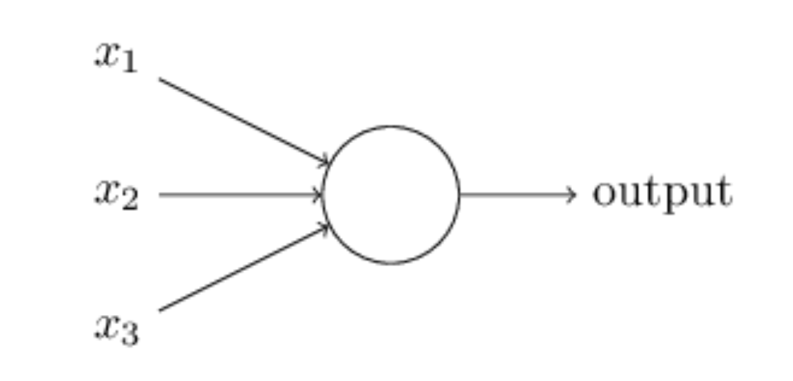
The field of artificial neural networks has a long history of development, and is closely connected with the advancement of computer science and computers in general. A model of artificial neurons was first developed by McCulloch and Pitts in 1943 to study signal processing in the brain and has later been refined by others. The general idea is to mimic neural networks in the human brain, which is composed of billions of neurons that communicate with each other by sending electrical signals. Each neuron accumulates its incoming signals, which must exceed an activation threshold to yield an output. If the threshold is not overcome, the neuron remains inactive, i.e. has zero output.
This behaviour has inspired a simple mathematical model for an artificial neuron. $$ y = f\left(\sum_{i=1}^n w_ix_i\right) = f(u) $$ Here, the output \( y \) of the neuron is the value of its activation function, which have as input a weighted sum of signals \( x_i, \dots ,x_n \) received by \( n \) other neurons.
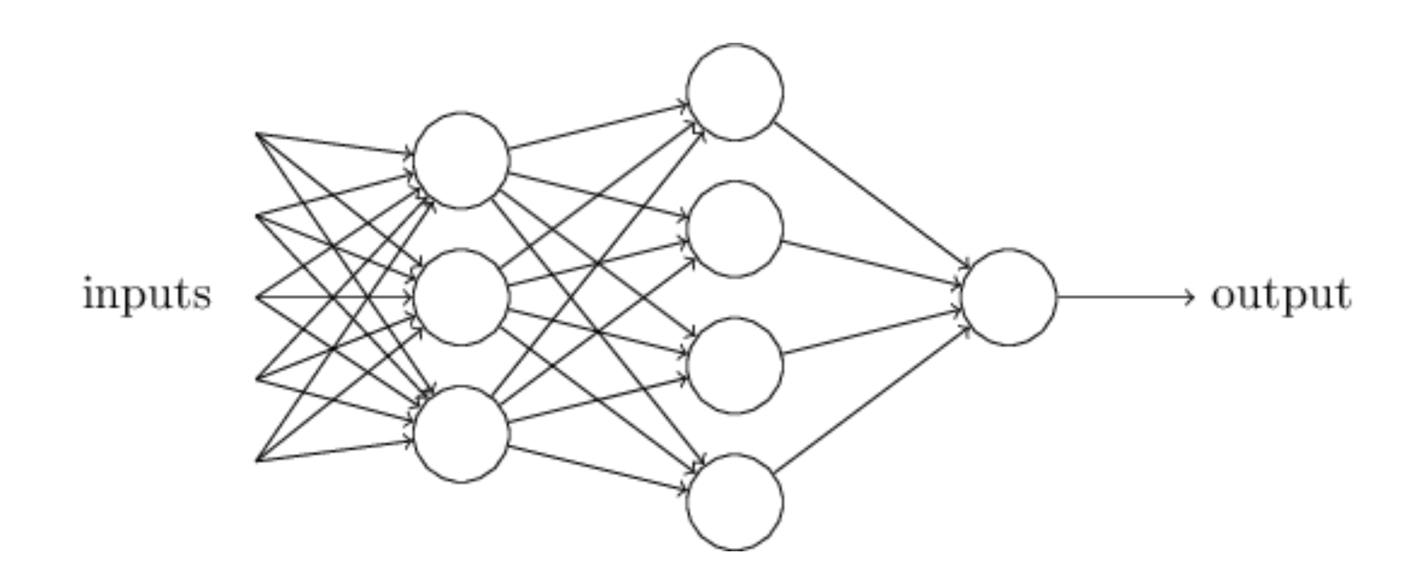
An artificial neural network (NN), is a computational model that consists of layers of connected neurons, or nodes. It is supposed to mimic a biological nervous system by letting each neuron interact with other neurons by sending signals in the form of mathematical functions between layers. A wide variety of different NNs have been developed, but most of them consist of an input layer, an output layer and eventual layers in-between, called hidden layers. All layers can contain an arbitrary number of nodes, and each connection between two nodes is associated with a weight variable.
The Hamiltonian of the quantum dot is given by $$ \hat{H} = \hat{H}_0 + \hat{V}, $$ where \( \hat{H}_0 \) is the many-body HO Hamiltonian, and \( \hat{V} \) is the inter-electron Coulomb interactions. In dimensionless units, $$ \hat{V}= \sum_{i < j}^N \frac{1}{r_{ij}}, $$ with \( r_{ij}=\sqrt{\mathbf{r}_i^2 - \mathbf{r}_j^2} \).
This leads to the separable Hamiltonian, with the relative motion part given by (\( r_{ij}=r \)) $$ \hat{H}_r=-\nabla^2_r + \frac{1}{4}\omega^2r^2+ \frac{1}{r}, $$ plus a standard Harmonic Oscillator problem for the center-of-mass motion. This system has analytical solutions in two and three dimensions (M. Taut 1993 and 1994).
Given a hamiltonian \( H \) and a trial wave function \( \Psi_T \), the variational principle states that the expectation value of \( \langle H \rangle \), defined through $$ \langle E \rangle = \frac{\int d\boldsymbol{R}\Psi^{\ast}_T(\boldsymbol{R})H(\boldsymbol{R})\Psi_T(\boldsymbol{R})} {\int d\boldsymbol{R}\Psi^{\ast}_T(\boldsymbol{R})\Psi_T(\boldsymbol{R})}, $$ is an upper bound to the ground state energy \( E_0 \) of the hamiltonian \( H \), that is $$ E_0 \le \langle H \rangle . $$ In general, the integrals involved in the calculation of various expectation values are multi-dimensional ones. Traditional integration methods such as the Gauss-Legendre will not be adequate for say the computation of the energy of a many-body system.
Choose a trial wave function \( \psi_T(\boldsymbol{R}) \). $$ P(\boldsymbol{R},\boldsymbol{\alpha})= \frac{\left|\psi_T(\boldsymbol{R},\boldsymbol{\alpha})\right|^2}{\int \left|\psi_T(\boldsymbol{R},\boldsymbol{\alpha})\right|^2d\boldsymbol{R}}. $$ This is our model, or likelihood/probability distribution function (PDF). It depends on some variational parameters \( \boldsymbol{\alpha} \). The approximation to the expectation value of the Hamiltonian is now $$ \langle E[\boldsymbol{\alpha}] \rangle = \frac{\int d\boldsymbol{R}\Psi^{\ast}_T(\boldsymbol{R},\boldsymbol{\alpha})H(\boldsymbol{R})\Psi_T(\boldsymbol{R},\boldsymbol{\alpha})} {\int d\boldsymbol{R}\Psi^{\ast}_T(\boldsymbol{R},\boldsymbol{\alpha})\Psi_T(\boldsymbol{R},\boldsymbol{\alpha})}. $$
$$ E_L(\boldsymbol{R},\boldsymbol{\alpha})=\frac{1}{\psi_T(\boldsymbol{R},\boldsymbol{\alpha})}H\psi_T(\boldsymbol{R},\boldsymbol{\alpha}), $$ called the local energy, which, together with our trial PDF yields $$ E[\boldsymbol{\alpha}]=\int P(\boldsymbol{R})E_L(\boldsymbol{R},\boldsymbol{\alpha}) d\boldsymbol{R}\approx \frac{1}{N}\sum_{i=1}^NE_L(\boldsymbol{R_i},\boldsymbol{\alpha}) $$ with \( N \) being the number of Monte Carlo samples.
The Algorithm for performing a variational Monte Carlo calculations runs thus as this
We want to perform a Variational Monte Carlo calculation of the ground state of two electrons in a quantum dot well with different oscillator energies, assuming total spin \( S=0 \). Our trial wave function has the following form $$ \begin{equation} \psi_{T}(\boldsymbol{r}_1,\boldsymbol{r}_2) = C\exp{\left(-\alpha_1\omega(r_1^2+r_2^2)/2\right)} \exp{\left(\frac{r_{12}}{(1+\alpha_2 r_{12})}\right)}, \label{eq:trial} \end{equation} $$ where the $\alpha$s represent our variational parameters, two in this case.
Why does the trial function look like this? How did we get there? This will be our main motivation for switching to Machine Learning.
To find an ansatz for the correlated part of the wave function, it is useful to rewrite the two-particle local energy in terms of the relative and center-of-mass motion. Let us denote the distance between the two electrons as \( r_{12} \). We omit the center-of-mass motion since we are only interested in the case when \( r_{12} \rightarrow 0 \). The contribution from the center-of-mass (CoM) variable \( \boldsymbol{R}_{\mathrm{CoM}} \) gives only a finite contribution. We focus only on the terms that are relevant for \( r_{12} \) and for three dimensions. The relevant local energy becomes then $$ \lim_{r_{12} \rightarrow 0}E_L(R)= \frac{1}{{\cal R}_T(r_{12})}\left(2\frac{d^2}{dr_{ij}^2}+\frac{4}{r_{ij}}\frac{d}{dr_{ij}}+ \frac{2}{r_{ij}}-\frac{l(l+1)}{r_{ij}^2}+2E \right){\cal R}_T(r_{12}) = 0. $$ Set \( l=0 \) and we have the so-called cusp condition $$ \frac{d {\cal R}_T(r_{12})}{dr_{12}} = -\frac{1}{2(l+1)} {\cal R}_T(r_{12})\qquad r_{12}\to 0 $$
# Importing various packages
from math import exp, sqrt
from random import random, seed
import numpy as np
import matplotlib.pyplot as plt
from mpl_toolkits.mplot3d import Axes3D
from matplotlib import cm
from matplotlib.ticker import LinearLocator, FormatStrFormatter
import sys

#Trial wave function for quantum dots in two dims
def WaveFunction(r,alpha,beta):
    r1 = r[0,0]**2 + r[0,1]**2
    r2 = r[1,0]**2 + r[1,1]**2
    r12 = sqrt((r[0,0]-r[1,0])**2 + (r[0,1]-r[1,1])**2)
    deno = r12/(1+beta*r12)
    return exp(-0.5*alpha*(r1+r2)+deno)

#Local energy  for quantum dots in two dims, using analytical local energy
def LocalEnergy(r,alpha,beta):

    r1 = (r[0,0]**2 + r[0,1]**2)
    r2 = (r[1,0]**2 + r[1,1]**2)
    r12 = sqrt((r[0,0]-r[1,0])**2 + (r[0,1]-r[1,1])**2)
    deno = 1.0/(1+beta*r12)
    deno2 = deno*deno
    return 0.5*(1-alpha*alpha)*(r1 + r2) +2.0*alpha + 1.0/r12+deno2*(alpha*r12-deno2+2*beta*deno-1.0/r12)

# The Monte Carlo sampling with the Metropolis algo
def MonteCarloSampling():

    NumberMCcycles= 100000
    StepSize = 1.0
    # positions
    PositionOld = np.zeros((NumberParticles,Dimension), np.double)
    PositionNew = np.zeros((NumberParticles,Dimension), np.double)
    # seed for rng generator
    seed()
    # start variational parameter
    alpha = 0.9
    for ia in range(MaxVariations):
        alpha += .025
        AlphaValues[ia] = alpha
        beta = 0.2
        for jb in range(MaxVariations):
            beta += .01
            BetaValues[jb] = beta
            energy = energy2 = 0.0
            DeltaE = 0.0
            #Initial position
            for i in range(NumberParticles):
                for j in range(Dimension):
                    PositionOld[i,j] = StepSize * (random() - .5)
            wfold = WaveFunction(PositionOld,alpha,beta)

            #Loop over MC MCcycles
            for MCcycle in range(NumberMCcycles):
                #Trial position
                for i in range(NumberParticles):
                    for j in range(Dimension):
                        PositionNew[i,j] = PositionOld[i,j] + StepSize * (random() - .5)
                wfnew = WaveFunction(PositionNew,alpha,beta)

                #Metropolis test to see whether we accept the move
                if random() < wfnew**2 / wfold**2:
                   PositionOld = PositionNew.copy()
                   wfold = wfnew
                   DeltaE = LocalEnergy(PositionOld,alpha,beta)
                energy += DeltaE
                energy2 += DeltaE**2

            #We calculate mean, variance and error ...
            energy /= NumberMCcycles
            energy2 /= NumberMCcycles
            variance = energy2 - energy**2
            error = sqrt(variance/NumberMCcycles)
            Energies[ia,jb] = energy
    return Energies, AlphaValues, BetaValues


#Here starts the main program with variable declarations
NumberParticles = 2
Dimension = 2
MaxVariations = 10
Energies = np.zeros((MaxVariations,MaxVariations))
AlphaValues = np.zeros(MaxVariations)
BetaValues = np.zeros(MaxVariations)
(Energies, AlphaValues, BetaValues) = MonteCarloSampling()

# Prepare for plots
fig = plt.figure()
ax = fig.gca(projection='3d')
# Plot the surface.
X, Y = np.meshgrid(AlphaValues, BetaValues)
surf = ax.plot_surface(X, Y, Energies,cmap=cm.coolwarm,linewidth=0, antialiased=False)
# Customize the z axis.
zmin = np.matrix(Energies).min()
zmax = np.matrix(Energies).max()
ax.set_zlim(zmin, zmax)
ax.set_xlabel(r'$\alpha$')
ax.set_ylabel(r'$\beta$')
ax.set_zlabel(r'$\langle E \rangle$')
ax.zaxis.set_major_locator(LinearLocator(10))
ax.zaxis.set_major_formatter(FormatStrFormatter('%.02f'))
# Add a color bar which maps values to colors.
fig.colorbar(surf, shrink=0.5, aspect=5)
plt.show()
The above procedure is not the smartest one. Looping over all variational parameters becomes expensive. Also, we don't use importance sampling and optimizations of the standard deviation (blocking, bootstrap, jackknife). Such codes are included in the above Github address.
We can also be smarter and use minimization methods to find the optimal variational parameters with fewer Monte Carlo cycles and then fire up our heavy artillery.
One way to achieve this is to minimize the energy as function of the variational parameters.
To find the derivatives of the local energy expectation value as function of the variational parameters, we can use the chain rule and the hermiticity of the Hamiltonian.
Let us define $$ \bar{E}_{\alpha_i}=\frac{d\langle E_L\rangle}{d\alpha_i}. $$ as the derivative of the energy with respect to the variational parameter \( \alpha_i \) We define also the derivative of the trial function (skipping the subindex \( T \)) as $$ \bar{\Psi}_{i}=\frac{d\Psi}{d\alpha_i}. $$
The elements of the gradient of the local energy are then (using the chain rule and the hermiticity of the Hamiltonian) $$ \bar{E}_{i}= 2\left( \langle \frac{\bar{\Psi}_{i}}{\Psi}E_L\rangle -\langle \frac{\bar{\Psi}_{i}}{\Psi}\rangle\langle E_L \rangle\right). $$ From a computational point of view it means that you need to compute the expectation values of $$ \langle \frac{\bar{\Psi}_{i}}{\Psi}E_L\rangle, $$ and $$ \langle \frac{\bar{\Psi}_{i}}{\Psi}\rangle\langle E_L\rangle $$ These integrals are evaluted using MC intergration (with all its possible error sources). We can then use methods like stochastic gradient or other minimization methods to find the optimal variational parameters (I don't discuss this topic here, but these methods are very important in ML).
We have a model, our likelihood function.
How should we define the cost function?
Suppose the trial function (our model) is the exact wave function. The action of the hamiltionan on the wave function $$ H\Psi = \mathrm{constant}\times \Psi, $$ The integral which defines various expectation values involving moments of the hamiltonian becomes then $$ \langle E^n \rangle = \langle H^n \rangle = \frac{\int d\boldsymbol{R}\Psi^{\ast}(\boldsymbol{R})H^n(\boldsymbol{R})\Psi(\boldsymbol{R})} {\int d\boldsymbol{R}\Psi^{\ast}(\boldsymbol{R})\Psi(\boldsymbol{R})}= \mathrm{constant}\times\frac{\int d\boldsymbol{R}\Psi^{\ast}(\boldsymbol{R})\Psi(\boldsymbol{R})} {\int d\boldsymbol{R}\Psi^{\ast}(\boldsymbol{R})\Psi(\boldsymbol{R})}=\mathrm{constant}. $$ This gives an important information: If I want the variance, the exact wave function leads to zero variance! The variance is defined as $$ \sigma_E = \langle E^2\rangle - \langle E\rangle^2. $$ Variation is then performed by minimizing both the energy and the variance.
We can then take the derivatives of $$ \sigma_E = \langle E^2\rangle - \langle E\rangle^2, $$ with respect to the variational parameters. The derivatives of the variance can then be used to defined the so-called Hessian matrix, which in turn allows us to use minimization methods like Newton's method or standard gradient methods.
This leads to however a more complicated expression, with obvious errors when evaluating integrals by Monte Carlo integration. Less used, see however Filippi and Umrigar. The expression becomes complicated $$ \bar{E}_{ij} = 2\left[ \langle (\frac{\bar{\Psi}_{ij}}{\Psi}+\frac{\bar{\Psi}_{j}}{\Psi}\frac{\bar{\Psi}_{i}}{\Psi})(E_L-\langle E\rangle)\rangle -\langle \frac{\bar{\Psi}_{i}}{\Psi}\rangle\bar{E}_j-\langle \frac{\bar{\Psi}_{j}}{\Psi}\rangle\bar{E}_i\right] +\langle \frac{\bar{\Psi}_{i}}{\Psi}E_L{_j}\rangle +\langle \frac{\bar{\Psi}_{j}}{\Psi}E_L{_i}\rangle -\langle \frac{\bar{\Psi}_{i}}{\Psi}\rangle\langle E_L{_j}\rangle \langle \frac{\bar{\Psi}_{j}}{\Psi}\rangle\langle E_L{_i}\rangle. $$
Evaluating the cost function means having to evaluate the above second derivative of the energy.
What is known as restricted Boltzmann Machines (RMB) have received a lot of attention lately. One of the major reasons is that they can be stacked layer-wise to build deep neural networks that capture complicated statistics.
The original RBMs had just one visible layer and a hidden layer, but recently so-called Gaussian-binary RBMs have gained quite some popularity in imaging since they are capable of modeling continuous data that are common to natural images.
Furthermore, they have been used to solve complicated quantum mechanical many-particle problems or classical statistical physics problems like the Ising and Potts classes of models.
Why use a generative model rather than the more well known discriminative deep neural networks (DNN)?
A BM is what we would call an undirected probabilistic graphical model with stochastic continuous or discrete units.
It is interpreted as a stochastic recurrent neural network where the state of each unit(neurons/nodes) depends on the units it is connected to. The weights in the network represent thus the strength of the interaction between various units/nodes.
It turns into a Hopfield network if we choose deterministic rather than stochastic units. In contrast to a Hopfield network, a BM is a so-called generative model. It allows us to generate new samples from the learned distribution.
A standard BM network is divided into a set of observable and visible units \( \hat{x} \) and a set of unknown hidden units/nodes \( \hat{h} \).
Additionally there can be bias nodes for the hidden and visible layers. These biases are normally set to \( 1 \).
BMs are stackable, meaning they cwe can train a BM which serves as input to another BM. We can construct deep networks for learning complex PDFs. The layers can be trained one after another, a feature which makes them popular in deep learning
However, they are often hard to train. This leads to the introduction of so-called restricted BMs, or RBMS. Here we take away all lateral connections between nodes in the visible layer as well as connections between nodes in the hidden layer. The network is illustrated in the figure below.
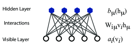
The network layers:
The goal of the hidden layer is to increase the model's expressive power. We encode complex interactions between visible variables by introducing additional, hidden variables that interact with visible degrees of freedom in a simple manner, yet still reproduce the complex correlations between visible degrees in the data once marginalized over (integrated out).
Examples of this trick being employed in physics:
The restricted Boltzmann machine is described by a Boltzmann distribution $$ \begin{align} P_{rbm}(\mathbf{x},\mathbf{h}) = \frac{1}{Z} e^{-\frac{1}{T_0}E(\mathbf{x},\mathbf{h})}, \label{_auto1} \end{align} $$ where \( Z \) is the normalization constant or partition function, defined as $$ \begin{align} Z = \int \int e^{-\frac{1}{T_0}E(\mathbf{x},\mathbf{h})} d\mathbf{x} d\mathbf{h}. \label{_auto2} \end{align} $$ It is common to ignore \( T_0 \) by setting it to one.
The function \( E(\mathbf{x},\mathbf{h}) \) gives the energy of a configuration (pair of vectors) \( (\mathbf{x}, \mathbf{h}) \). The lower the energy of a configuration, the higher the probability of it. This function also depends on the parameters \( \mathbf{a} \), \( \mathbf{b} \) and \( W \). Thus, when we adjust them during the learning procedure, we are adjusting the energy function to best fit our problem.
An expression for the energy function is $$ E(\hat{x},\hat{h}) = -\sum_{ia}^{NA}b_i^a \alpha_i^a(x_i)-\sum_{jd}^{MD}c_j^d \beta_j^d(h_j)-\sum_{ijad}^{NAMD}b_i^a \alpha_i^a(x_i)c_j^d \beta_j^d(h_j)w_{ij}^{ad}. $$
Here \( \beta_j^d(h_j) \) and \( \alpha_i^a(x_j) \) are so-called transfer functions that map a given input value to a desired feature value. The labels \( a \) and \( d \) denote that there can be multiple transfer functions per variable. The first sum depends only on the visible units. The second on the hidden ones. Note that there is no connection between nodes in a layer.
The quantities \( b \) and \( c \) can be interpreted as the visible and hidden biases, respectively.
The connection between the nodes in the two layers is given by the weights \( w_{ij} \).
RBMs were first developed using binary units in both the visible and hidden layer. The corresponding energy function is defined as follows: $$ \begin{align} E(\mathbf{x}, \mathbf{h}) = - \sum_i^M x_i a_i- \sum_j^N b_j h_j - \sum_{i,j}^{M,N} x_i w_{ij} h_j, \label{_auto3} \end{align} $$ where the binary values taken on by the nodes are most commonly 0 and 1.
Another varient is the RBM where the visible units are Gaussian while the hidden units remain binary: $$ \begin{align} E(\mathbf{x}, \mathbf{h}) = \sum_i^M \frac{(x_i - a_i)^2}{2\sigma_i^2} - \sum_j^N b_j h_j - \sum_{i,j}^{M,N} \frac{x_i w_{ij} h_j}{\sigma_i^2}. \label{_auto4} \end{align} $$
Metropolis sampling starts by suggesting a new configuration \( \boldsymbol{x}^{k+1} \). In the brute force method this is done by some random change of the visible units. The new configuration is then accepted with the acceptance probability $$ \begin{align} A(\boldsymbol{x}^k \rightarrow \boldsymbol{x}^{k+1}) = \text{min} (1, \frac{P(\boldsymbol{x}^{k+1})}{P(\boldsymbol{x}^k)}), \label{_auto5} \end{align} $$ where we need the marginalized probability $$ \begin{align} P(\boldsymbol{x}) &= \sum_\mathbf{h} P_{rbm}(\mathbf{x}, \mathbf{h}) \label{_auto6}\\ &= \frac{1}{Z}\sum_\mathbf{h} e^{-E(\mathbf{x}, \mathbf{h})}. \label{_auto7} \end{align} $$
In this method we sample from the joint probability \( P_{rbm} (\mathbf{x}, \mathbf{h}) \) by way of a two step sampling process. We alternately update the visible and hidden units. New samples are generated according to the conditional probabilities \( P(x_i|\mathbf{h}) \) and \( P(h_j|\mathbf{x}) \) respectively and accepted with the probability of \( 1 \). While the the visible nodes are dependent on the hidden nodes and vice versa, the nodes are independent of other nodes within the same layer. This is due to there being no intra layer interactions in the restricted Boltzmann machine.
The conditional probabilities are often referred to as the activitation functions in the neural networks context due to their role in determining the node outputs. For the binary-binary RBM they are $$ \begin{align} P(h_j = 1 | \boldsymbol{x}) &= \frac{1}{1 + e^{-b_j - \sum_i x_i w_{ij}}} \label{_auto8}\\ P(x_i = 1 | \boldsymbol{h}) &= \frac{1}{1 + e^{-a_j - \sum_j h_j w_{ij}}}, \label{_auto9} \end{align} $$ where we recognize the logistic sigmoid function \( \sigma (x) = 1/(1+exp(-x)) \).
When working with a training dataset, the most common training approach is maximizing the log-likelihood of the training data. The log likelihood characterizes the log-probability of generating the observed data using our generative model. Using this method our cost function is chosen as the negative log-likelihood. The learning then consists of trying to find parameters that maximize the probability of the dataset, and is known as Maximum Likelihood Estimation (MLE). Denoting the parameters as \( \boldsymbol{\theta} = a_1,...,a_M,b_1,...,b_N,w_{11},...,w_{MN} \), the log-likelihood is given by $$ \begin{align} \mathcal{L}(\{ \theta_i \}) &= \langle \text{log} P_\theta(\boldsymbol{x}) \rangle_{data} \label{_auto12}\\ &= - \langle E(\boldsymbol{x}; \{ \theta_i\}) \rangle_{data} - \text{log} Z(\{ \theta_i\}), \label{_auto13} \end{align} $$ where we used that the normalization constant does not depend on the data, \( \langle \text{log} Z(\{ \theta_i\}) \rangle = \text{log} Z(\{ \theta_i\}) \) Our cost function is the negative log-likelihood, \( \mathcal{C}(\{ \theta_i \}) = - \mathcal{L}(\{ \theta_i \}) \)
The training procedure of choice often is Stochastic Gradient Descent (SGD). It consists of a series of iterations where we update the parameters according to the equation $$ \begin{align} \boldsymbol{\theta}_{k+1} = \boldsymbol{\theta}_k - \eta \nabla \mathcal{C} (\boldsymbol{\theta}_k) \label{_auto14} \end{align} $$ at each \( k \)-th iteration. There are a range of variants of the algorithm which aim at making the learning rate \( \eta \) more adaptive so the method might be more efficient while remaining stable.
We now need the gradient of the cost function in order to minimize it. We find that $$ \begin{align} \frac{\partial \mathcal{C}(\{ \theta_i\})}{\partial \theta_i} &= \langle \frac{\partial E(\boldsymbol{x}; \theta_i)}{\partial \theta_i} \rangle_{data} + \frac{\partial \text{log} Z(\{ \theta_i\})}{\partial \theta_i} \label{_auto15}\\ &= \langle O_i(\boldsymbol{x}) \rangle_{data} - \langle O_i(\boldsymbol{x}) \rangle_{model}, \label{_auto16} \end{align} $$ where in order to simplify notation we defined the "operator" $$ \begin{align} O_i(\boldsymbol{x}) = \frac{\partial E(\boldsymbol{x}; \theta_i)}{\partial \theta_i}, \label{_auto17} \end{align} $$ and used the statistical mechanics relationship between expectation values and the log-partition function: $$ \begin{align} \langle O_i(\boldsymbol{x}) \rangle_{model} = \text{Tr} P_\theta(\boldsymbol{x})O_i(\boldsymbol{x}) = - \frac{\partial \text{log} Z(\{ \theta_i\})}{\partial \theta_i}. \label{_auto18} \end{align} $$
The data-dependent term in the gradient is known as the positive phase of the gradient, while the model-dependent term is known as the negative phase of the gradient. The aim of the training is to lower the energy of configurations that are near observed data points (increasing their probability), and raising the energy of configurations that are far from observed data points (decreasing their probability).
The gradient of the negative log-likelihood cost function of a Binary-Binary RBM is then $$ \begin{align} \frac{\partial \mathcal{C} (w_{ij}, a_i, b_j)}{\partial w_{ij}} =& \langle x_i h_j \rangle_{data} - \langle x_i h_j \rangle_{model} \label{_auto19}\\ \frac{\partial \mathcal{C} (w_{ij}, a_i, b_j)}{\partial a_{ij}} =& \langle x_i \rangle_{data} - \langle x_i \rangle_{model} \label{_auto20}\\ \frac{\partial \mathcal{C} (w_{ij}, a_i, b_j)}{\partial b_{ij}} =& \langle h_i \rangle_{data} - \langle h_i \rangle_{model}. \label{_auto21}\\ \label{_auto22} \end{align} $$ To get the expecation values with respect to the data, we set the visible units to each of the observed samples in the training data, then update the hidden units according to the conditional probability found before. We then average over all samples in the training data to calculate expectation values with respect to the data.
To get the expectation values with respect to the model, we use Gibbs sampling. We can either initialize the \( \boldsymbol{x} \) randomly or with a training sample. While we ideally want a large number of Gibbs iterations \( n\rightarrow n \), one might decide to truncate it earlier for efficiency. Doing this while having intialized \( \boldsymbol{x} \) with a training data vector is referred to as contrastive divergence (CD), because one is then closer to approximating the gradient of this function than the negative log-likelihood. The contrastive divergence function is the difference between two Kullback-Leibler divergences (also called relative entropy), which measure how one probability distribution diverges from a second, expected probability distribution (in this case the estimated one from the ground truth one).
The idea of applying RBMs to quantum many body problems was presented by G. Carleo and M. Troyer, working with ETH Zurich and Microsoft Research.
Some of their motivation included
Carleo and Troyer applied the RBM to the quantum mechanical spin lattice systems of the Ising model and Heisenberg model, with encouraging results. Our goal is to test the method on systems of moving particles. For the spin lattice systems it was natural to use a binary-binary RBM, with the nodes taking values of 1 and -1. For moving particles, on the other hand, we want the visible nodes to be continuous, representing position coordinates. Thus, we start by choosing a Gaussian-binary RBM, where the visible nodes are continuous and hidden nodes take on values of 0 or 1. If eventually we would like the hidden nodes to be continuous as well the rectified linear units seem like the most relevant choice.
You can find the codes for the simple two-electron case at the Github repository https://github.com/mhjensenseminars/MachineLearningTalk/tree/master/doc/Programs/MLcpp/src. Python codes to come, only c++ as of now.
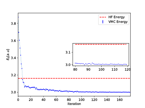
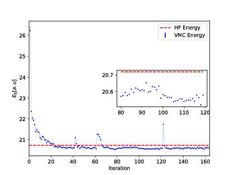
The trial wave function is based on the product of a Slater determinant with Gaussian orbitals, a simple Jastrow factor \( \exp{(r_{ij})} \) and the reduced Boltzmann machines.
The Broyden-Fletcher-Goldfarb-Shanno algorithm was used for the minimization. We used \( 14 \) hidden nodes in the calculations below.
When the goal of the training is to approximate a probability distribution, as it is in generative modeling, another relevant measure is the Kullback-Leibler divergence, also known as the relative entropy or Shannon entropy. It is a non-symmetric measure of the dissimilarity between two probability density functions \( p \) and \( q \). If \( p \) is the unkown probability which we approximate with \( q \), we can measure the difference by $$ \begin{align} \text{KL}(p||q) = \int_{-\infty}^{\infty} p (\boldsymbol{x}) \log \frac{p(\boldsymbol{x})}{q(\boldsymbol{x})} d\boldsymbol{x}. \label{_auto33} \end{align} $$
Thus, the Kullback-Leibler divergence between the distribution of the training data \( f(\boldsymbol{x}) \) and the model distribution \( p(\boldsymbol{x}| \boldsymbol{\theta}) \) is $$ \begin{align} \text{KL} (f(\boldsymbol{x})|| p(\boldsymbol{x}| \boldsymbol{\theta})) =& \int_{-\infty}^{\infty} f (\boldsymbol{x}) \log \frac{f(\boldsymbol{x})}{p(\boldsymbol{x}| \boldsymbol{\theta})} d\boldsymbol{x} \label{_auto34}\\ =& \int_{-\infty}^{\infty} f(\boldsymbol{x}) \log f(\boldsymbol{x}) d\boldsymbol{x} - \int_{-\infty}^{\infty} f(\boldsymbol{x}) \log p(\boldsymbol{x}| \boldsymbol{\theta}) d\boldsymbol{x} \label{_auto35}\\ %=& \mathbb{E}_{f(\boldsymbol{x})} (\log f(\boldsymbol{x})) - \mathbb{E}_{f(\boldsymbol{x})} (\log p(\boldsymbol{x}| \boldsymbol{\theta})) =& \langle \log f(\boldsymbol{x}) \rangle_{f(\boldsymbol{x})} - \langle \log p(\boldsymbol{x}| \boldsymbol{\theta}) \rangle_{f(\boldsymbol{x})} \label{_auto36}\\ =& \langle \log f(\boldsymbol{x}) \rangle_{data} + \langle E(\boldsymbol{x}) \rangle_{data} + \log Z \label{_auto37}\\ =& \langle \log f(\boldsymbol{x}) \rangle_{data} + \mathcal{C}_{LL} . \label{_auto38} \end{align} $$
The first term is constant with respect to \( \boldsymbol{\theta} \) since \( f(\boldsymbol{x}) \) is independent of \( \boldsymbol{\theta} \). Thus the Kullback-Leibler Divergence is minimal when the second term is minimal. The second term is the log-likelihood cost function, hence minimizing the Kullback-Leibler divergence is equivalent to maximizing the log-likelihood.
To further understand generative models it is useful to study the gradient of the cost function which is needed in order to minimize it using methods like stochastic gradient descent.
The partition function is the generating function of expectation values, in particular there are mathematical relationships between expectation values and the log-partition function. In this case we have $$ \begin{align} \langle \frac{ \partial E(\boldsymbol{x}; \theta_i) } { \partial \theta_i} \rangle_{model} = \int p(\boldsymbol{x}| \boldsymbol{\theta}) \frac{ \partial E(\boldsymbol{x}; \theta_i) } { \partial \theta_i} d\boldsymbol{x} = -\frac{\partial \log Z(\theta_i)}{ \partial \theta_i} . \label{_auto39} \end{align} $$
Here \( \langle \cdot \rangle_{model} \) is the expectation value over the model probability distribution \( p(\boldsymbol{x}| \boldsymbol{\theta}) \).
Using the previous relationship we can express the gradient of the cost function as $$ \begin{align} \frac{\partial \mathcal{C}_{LL}}{\partial \theta_i} =& \langle \frac{ \partial E(\boldsymbol{x}; \theta_i) } { \partial \theta_i} \rangle_{data} + \frac{\partial \log Z(\theta_i)}{ \partial \theta_i} \label{_auto40}\\ =& \langle \frac{ \partial E(\boldsymbol{x}; \theta_i) } { \partial \theta_i} \rangle_{data} - \langle \frac{ \partial E(\boldsymbol{x}; \theta_i) } { \partial \theta_i} \rangle_{model} \label{_auto41}\\ %=& \langle O_i(\boldsymbol{x}) \rangle_{data} - \langle O_i(\boldsymbol{x}) \rangle_{model} \label{_auto42} \end{align} $$
This expression shows that the gradient of the log-likelihood cost function is a difference of moments, with one calculated from the data and one calculated from the model. The data-dependent term is called the positive phase and the model-dependent term is called the negative phase of the gradient. We see now that minimizing the cost function results in lowering the energy of configurations \( \boldsymbol{x} \) near points in the training data and increasing the energy of configurations not observed in the training data. That means we increase the model's probability of configurations similar to those in the training data.
The gradient of the cost function also demonstrates why gradients of unsupervised, generative models must be computed differently from for those of for example FNNs. While the data-dependent expectation value is easily calculated based on the samples \( \boldsymbol{x}_i \) in the training data, we must sample from the model in order to generate samples from which to caclulate the model-dependent term. We sample from the model by using MCMC-based methods. We can not sample from the model directly because the partition function \( Z \) is generally intractable.
As in supervised machine learning problems, the goal is also here to perform well on unseen data, that is to have good generalization from the training data. The distribution \( f(x) \) we approximate is not the true distribution we wish to estimate, it is limited to the training data. Hence, in unsupervised training as well it is important to prevent overfitting to the training data. Thus it is common to add regularizers to the cost function in the same manner as we discussed for say linear regression.