Machine learning and quantum computing in physics research and education
The 30th Anniversary Symposium of the Center for Computational Sciences at the University of Tsukuba, October 13-14, 2022
What is this talk about?
The main emphasis is to give you a short and pedestrian introduction to the whys and hows we can use (with several examples) machine learning methods and quantum technologies in physics. And why this could (or should) be of interest. I will also try to link to educational activities.
These slides are at https://mhjensenseminars.github.io/MachineLearningTalk/doc/pub/Tsukubasymposium/html/Tsukubasymposium-reveal.html
Basic activities, Overview
- Machine Learning applied to classical and quantum mechanical systems and analysis of physics experiments
- Quantum Engineering
- Quantum algorithms
- Quantum Machine Learning
- Educational initiatives
Many folks to thank
- MSU: Ben Hall, Jane Kim, Julie Butler, Danny Jammoa, Nicholas Cariello, Johannes Pollanen (Expt), Niyaz Beysengulov (Expt), Dean Lee, Scott Bogner, Heiko Hergert, Matt Hirn, Huey-Wen Lin, Alexei Bazavov, Andrea Shindler and Angela Wilson
- UiO: Stian Bilek, Heine Åbø (OsloMet), Håkon Emil Kristiansen, Øyvind Schøyen Sigmundsson, Jonas Boym Flaten, Linus Ekstrøm, Oskar Leinoen, Kristian Wold (OsloMet), Lasse Vines (Expt) Andrej Kuznetsov (Expt), David Rivas Gongora (Expt) and Marianne Bathen (Expt, now PD at ETH)
This work is supported by the U.S. Department of Energy, Office of Science, office of Nuclear Physics under grant No. DE-SC0021152 and U.S. National Science Foundation Grants No. PHY-1404159 and PHY-2013047 and the Norwegian ministry of Education and Research for PhD fellowships.
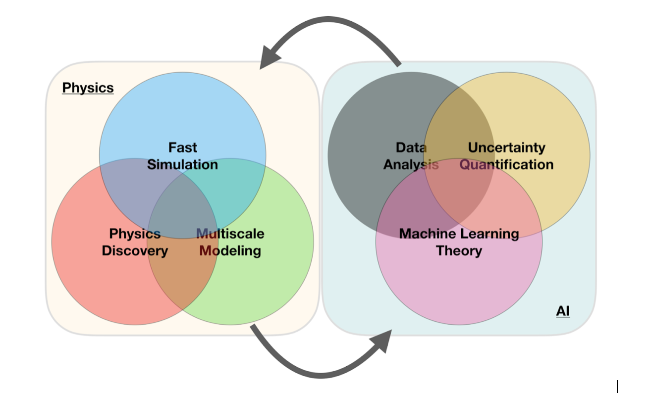
A simple perspective on the interface between ML and Physics
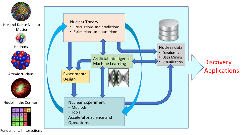
ML in Nuclear Physics
AI/ML and some statements you may have heard (and what do they mean?)
- Fei-Fei Li on ImageNet: map out the entire world of objects (The data that transformed AI research)
- Russell and Norvig in their popular textbook: relevant to any intellectual task; it is truly a universal field (Artificial Intelligence, A modern approach)
- Woody Bledsoe puts it more bluntly: in the long run, AI is the only science (quoted in Pamilla McCorduck, Machines who think)
If you wish to have a critical read on AI/ML from a societal point of view, see Kate Crawford's recent text Atlas of AI
Here: with AI/ML we intend a collection of machine learning methods with an emphasis on statistical learning and data analysisScientific Machine Learning
An important and emerging field is what has been dubbed as scientific ML, see the article by Deiana et al Applications and Techniques for Fast Machine Learning in Science, arXiv:2110.13041
The authors discuss applications and techniques for fast machine learning (ML) in science – the concept of integrating power ML methods into the real-time experimental data processing loop to accelerate scientific discovery. The report covers three main areas
- applications for fast ML across a number of scientific domains;
- techniques for training and implementing performant and resource-efficient ML algorithms;
- and computing architectures, platforms, and technologies for deploying these algorithms.
Lots of room for creativity
Not all the algorithms and methods can be given a rigorous mathematical justification, opening up thereby for experimenting and trial and error and thereby exciting new developments.
A solid command of linear algebra, multivariate theory, probability theory, statistical data analysis, optimization algorithms, understanding errors and Monte Carlo methods is important in order to understand many of the various algorithms and methods.
Job market, a personal statement: A familiarity with ML is almost becoming a prerequisite for many of the most exciting employment opportunities. And add quantum computing and there you are!
Types of machine learning
The approaches to machine learning are many, but are often split into two main categories. In supervised learning we know the answer to a problem, and let the computer deduce the logic behind it. On the other hand, unsupervised learning is a method for finding patterns and relationship in data sets without any prior knowledge of the system. Some authours also operate with a third category, namely reinforcement learning. This is a paradigm of learning inspired by behavioural psychology, where learning is achieved by trial-and-error, solely from rewards and punishment.
Another way to categorize machine learning tasks is to consider the desired output of a system. Some of the most common tasks are:
- Classification: Outputs are divided into two or more classes. The goal is to produce a model that assigns inputs into one of these classes. An example is to identify digits based on pictures of hand-written ones. Classification is typically supervised learning.
- Regression: Finding a functional relationship between an input data set and a reference data set. The goal is to construct a function that maps input data to continuous output values.
- Clustering: Data are divided into groups with certain common traits, without knowing the different groups beforehand. It is thus a form of unsupervised learning.
Machine learning and theory (physics): Why?
- ML tools can help us to speed up the scientific process cycle and hence facilitate discoveries
- Enabling fast emulation for big simulations
- Revealing the information content of measured observables w.r.t. theory
- Identifying crucial experimental data for better constraining theory
- Providing meaningful input to applications and planned measurements
- ML tools can help us to reveal the structure of our models
- Parameter estimation with heterogeneous/multi-scale datasets
- Model reduction
- ML tools can help us to provide predictive capability
- Theoretical results often involve ultraviolet and infrared extrapolations due to Hilbert-space truncations
- Uncertainty quantification essential
- Theoretical models are often applied to entirely new systems and conditions that are not accessible to experiment
Examples of Machine Learning methods and applications in physics
- Machine learning for data mining: Oftentimes, it is necessary to be able to accurately calculate observables that have not been measured, to supplement the existing databases.
- Density functional theory: Energy density functional calibration involving Bayesian optimization and deep learning ML. A promising avenue for ML applications is the emulation of DFT results.
- Nuclear physics properties with ML: Improving predictive power of nuclear models by emulating model residuals.
- Effective field theory and nuclear many-body systems: Truncation errors and low-energy coupling constant calibration, nucleon-nucleon scattering calculations, variational calculations with ANN for light nuclei, NN extrapolation of nuclear structure observables
- Nuclear shell model UQ: ML methods have been used to provide UQ of configuration interaction calculations.
Examples of Machine Learning methods and applications in physics, continues
- Low-energy nuclear reactions UQ: Bayesian optimization studies of the nucleon-nucleus optical potential, R-matrix analyses, and statistical spatial networks to study patterns in nuclear reaction networks.
- Neutron star properties and nuclear matter equation of state: constraining the equation of state by properties on neutron stars and selected properties of finite nuclei
- Experimental design: Bayesian ML provides a framework to maximize the success of on experiment based on the best information available on existing data, experimental conditions, and theoretical models.
More examples
The large amount of degrees of freedom pertain to both theory and experiment in physics. With increasingly complicated experiments that produce large amounts data, automated classification of events becomes increasingly important. Here, deep learning methods offer a plethora of interesting research avenues.
- Reconstruction of particle trajectories or classification of events are typical examples where ML methods are being used. However, since these data can often be extremely noisy, the precision necessary for discovery in physics requires algorithmic improvements. Research along such directions, interfacing nuclear physics with AI/ML is expected to play a significant role in physics discoveries related to new facilities. The treatment of corrupted data in imaging and image processing is also a relevant topic.
- Design of detectors represents an important area of applications for ML/AI methods in nuclear physics.
And more
- An important application of AI/ML methods is to improve the estimation of bias or uncertainty due to the introduction of or lack of physical constraints in various theoretical models.
- In theory, we expect to use AI/ML algorithms and methods to improve our knowledge about correlations of physical model parameters in data for quantum many-body systems. Deep learning methods show great promise in circumventing the exploding dimensionalities encountered in quantum mechanical many-body studies.
- Merging a frequentist approach (the standard path in ML theory) with a Bayesian approach, has the potential to infer better probabilitity distributions and error estimates. As an example, methods for fast Monte-Carlo- based Bayesian computation of nuclear density functionals show great promise.
- Machine Learning and Quantum Computing is a very interesting avenue to explore. See for example talk of Sofia Vallecorsa.
Selected references
- Mehta et al. and Physics Reports (2019).
- Machine Learning and the Physical Sciences by Carleo et al
- Ab initio solution of the many-electron Schrödinger equation with deep neural networks by Pfau et al.
- Report from the A.I. For Nuclear Physics Workshop by Bedaque et al., Eur J. Phys. A 57, (2021)
- Particle Data Group summary on ML methods
- And the BAND collaboration at https://bandframework.github.io/
Quantum Monte Carlo and deep learning
Given a hamiltonian \( H \) and a trial wave function \( \Psi_T \), the variational principle states that the expectation value of \( \langle H \rangle \), defined through
$$
\langle E \rangle =
\frac{\int d\boldsymbol{R}\Psi^{\ast}_T(\boldsymbol{R})H(\boldsymbol{R})\Psi_T(\boldsymbol{R})}
{\int d\boldsymbol{R}\Psi^{\ast}_T(\boldsymbol{R})\Psi_T(\boldsymbol{R})},
$$
is an upper bound to the ground state energy \( E_0 \) of the hamiltonian \( H \), that is
$$
E_0 \le \langle E \rangle.
$$
In general, the integrals involved in the calculation of various expectation values are multi-dimensional ones. Traditional integration methods such as Gaussian quadrature will not be adequate for say the computation of the energy of a many-body system. Basic philosophy: Let a neural network find the optimal wave function
Monte Carlo methods and Neural Networks
Machine Learning and the Deuteron by Kebble and Rios and Variational Monte Carlo calculations of \( A\le 4 \) nuclei with an artificial neural-network correlator ansatz by Adams et al.
Adams et al:
$$
\begin{align}
H_{LO} &=-\sum_i \frac{{\vec{\nabla}_i^2}}{2m_N}
+\sum_{i < j} {\left(C_1 + C_2\, \vec{\sigma_i}\cdot\vec{\sigma_j}\right)
e^{-r_{ij}^2\Lambda^2 / 4 }}
\nonumber\\
&+D_0 \sum_{i < j < k} \sum_{\text{cyc}}
{e^{-\left(r_{ik}^2+r_{ij}^2\right)\Lambda^2/4}}\,,
\tag{1}
\end{align}
$$
where \( m_N \) is the mass of the nucleon, \( \vec{\sigma_i} \) is the Pauli matrix acting on nucleon \( i \), and \( \sum_{\text{cyc}} \) stands for the cyclic permutation of \( i \), \( j \), and \( k \). The low-energy constants \( C_1 \) and \( C_2 \) are fit to the deuteron binding energy and to the neutron-neutron scattering length
Deep learning neural networks, Variational Monte Carlo calculations of \( A\le 4 \) nuclei with an artificial neural-network correlator ansatz by Adams et al.
An appealing feature of the neural network ansatz is that it is more general than the more conventional product of two- and three-body spin-independent Jastrow functions
$$
\begin{align}
|\Psi_V^J \rangle = \prod_{i < j < k} \Big( 1-\sum_{\text{cyc}} u(r_{ij}) u(r_{jk})\Big) \prod_{i < j} f(r_{ij}) | \Phi\rangle\,,
\tag{2}
\end{align}
$$
which is commonly used for nuclear Hamiltonians that do not contain tensor and spin-orbit terms. The above function is replaced by a four-layer Neural Network.
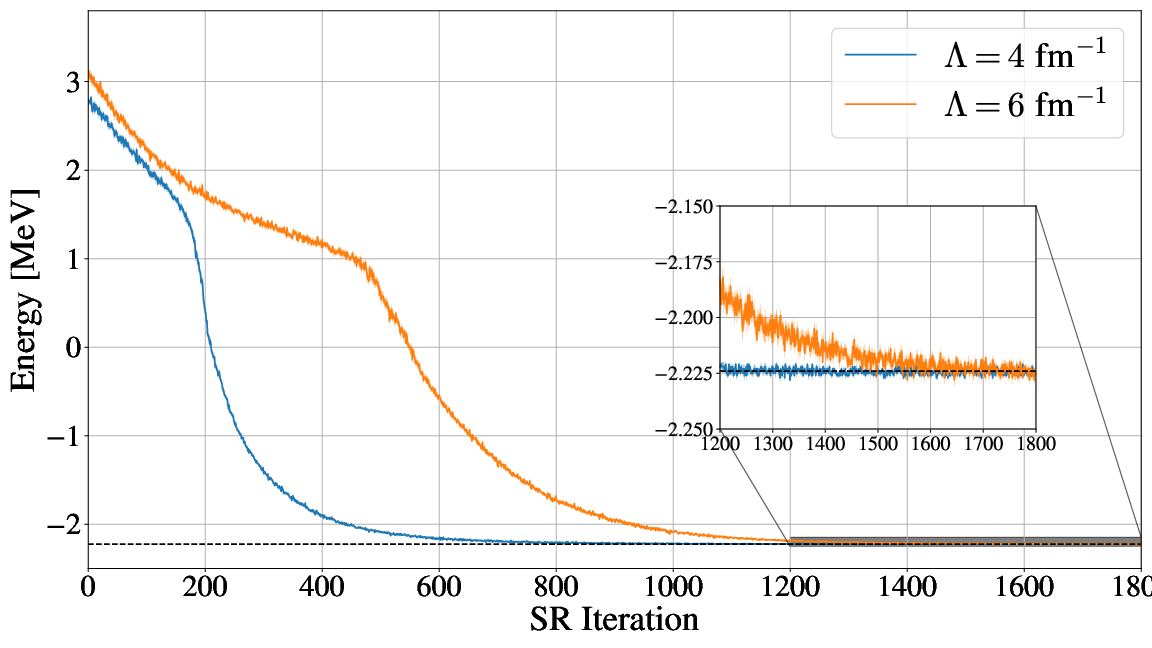
Gnech et al, Variational Monte Carlo calculations of \( A\le 6 \) nuclei Few Body Systems 63, (2022)

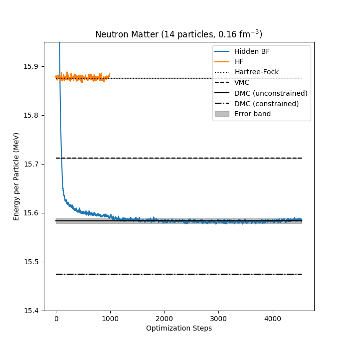
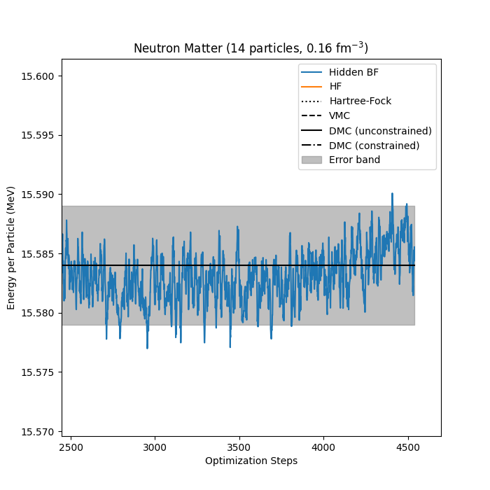
Neutron matter with \( N=14 \) neutron
Bryce Fore, Jane Kim, Alessandro Lovato and MHJ, in preparation
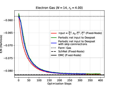
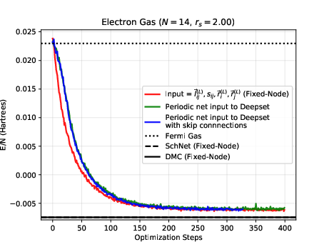
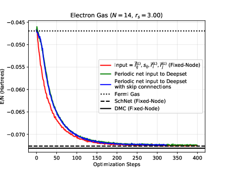
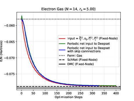
The electron gas in three dimensions with \( N=14 \) electrons (Wigner-Seitz radius \( r_s=4 \) Ry)
Jane Kim, Bryce Fore, Alessandro Lovato and MHJ, in preparation and Nordhagen, Kim, Fore, Lovato and MHJ, ArXiv 2210.00365
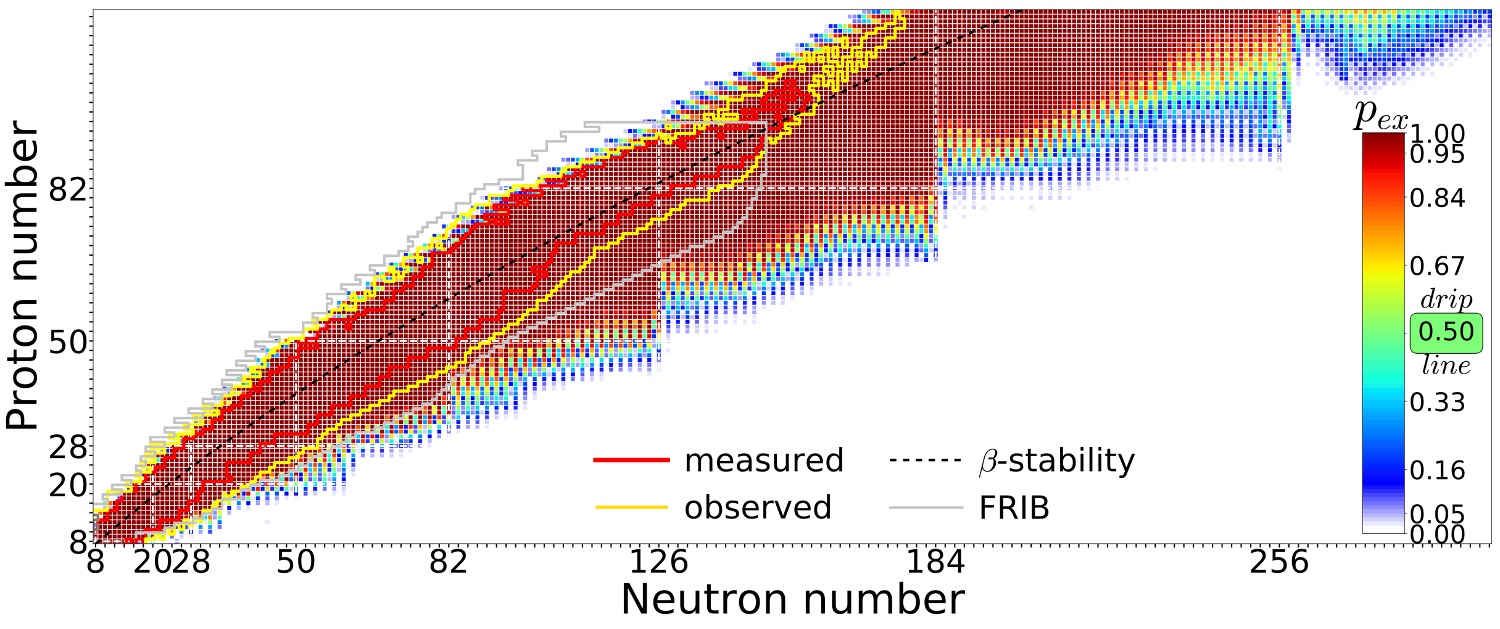
Quantified limits of the nuclear landscape
Neufcourt et al., Phys. Rev. C 101, 044307 (2020)Predictions made with eleven global mass model and Bayesian model averaging. Plot shows the probability of existence that the nucleus is bound with respect to proton and neutron decay.
Quantum Technologies
Quantum Engineering
- be scalable
- have qubits that can be entangled
- have reliable initializations protocols to a standard state
- have a set of universal quantum gates to control the quantum evolution
- have a coherence time much longer than the gate operation time
- have a reliable read-out mechanism for measuring the qubit states
- and many more
Candidate systems
- Superconducting Josephon junctions
- Single photons
- Trapped ions and atoms
- Nuclear Magnetic Resonance
- Quantum dots, expt at MSU
- Point Defects in semiconductors, experiments at UiO, center for Materials Science
- more
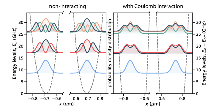
Electrons (quantum dots) on superfluid helium
Electrons on superfluid helium represent a promising platform for investigating strongly-coupled qubits.
Therefore, a systematic investigation of the controlled generation of entanglement between two trapped electrons under the influence of coherent microwave driving pulses, taking into account the effects of the Coulomb interaction between electrons, is of significant importance for quantum information processing using trapped electrons.
- Time-Dependent full configuration interaction theory
- Time-dependent Coupled-Cluster theory
- Designing quantum circuits
Electrons on superfluid helium
Beyzenguliov, Pollanen, MHJ and et al., in preparation
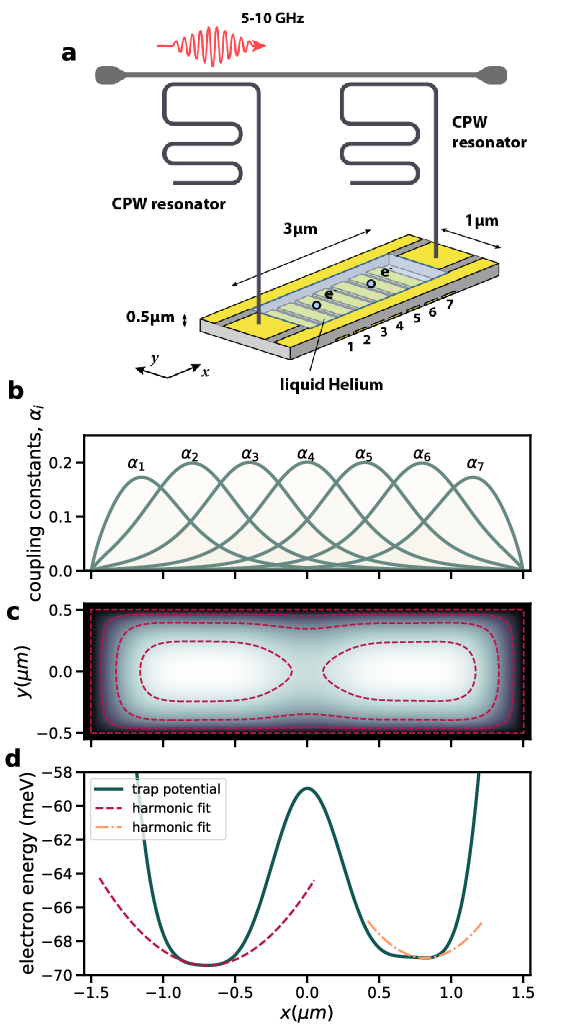
Electrons on superfluid helium, tuning wells
Beyzenguliov, Pollanen, MHJ and et al., in preparation
Education
- Incorporate elements of statistical data analysis and Machine Learning in undergraduate programs
- Develop courses on Machine Learning and statistical data analysis
- Build up a series of courses in QIS, inspiration QuSTEAM (Quantum Information Science, Technology, Engineering, Arts and Mathematics) initiative from USA
- Modifying contents of present Physics programs or new programs on Computational Physics and Quantum Technologies
- study direction/option in quantum technologies
- study direction/option in Artificial Intelligence and Machine Learning
- and more
QuSTEAM Model

Possible courses
- General university course on quantum mech and quantum technologies
- Information Systems
- From Classical Information theory to Quantum Information theory
- Classical vs. Quantum Logic
- Classical and Quantum Laboratory
- Discipline-Based Quantum Mechanics
- Quantum Software
- Quantum Hardware
- more
Important Issues to think of
- Lots of conceptual learning: superposition, entanglement, QIS applications, etc.
- Coding is indispensable. That is why this should be a part of a CS/DS program
- Teamwork, project management, and communication are important and highly valued
- Engagement with industry: guest lectures, virtual tours, co-ops, and/or internships.
Observations
- Students do not really know what QIS is.
- ML/AI seen as black boxes/magic!
- Students perceive that a graduate degree is necessary to work in QIS. A BSc will help.
Future Needs/Problems
- There are already great needs for specialized people (Ph. D. s, postdocs), but also needs of people with a broad overview of what is possible in ML/AI and/or QIS.
- There are not enough potential employees in AI/ML and QIS . It is a supply gap, not a skills gap.
- A BSc with specialization is a good place to start
- It is tremendously important to get everyone speaking the same language. Facility with the vernacular of quantum mechanics is a big plus.
- There is a huge list of areas where technical expertise may be important. But employers are often more concerned with attributes like project management, working well in a team, interest in the field, and adaptability than in specific technical skills.
Observations (or conclusions if you prefer)
- Need for AI/Machine Learning in physics, lots of ongoing activities
- To solve many complex problems and facilitate discoveries, multidisciplinary efforts efforts are required involving scientists in physics, statistics, computational science, applied math and other fields.
- There is a need for focused AI/ML learning efforts that will benefit accelerator science and experimental and theoretical programs
- How do we develop insights, competences, knowledge in statistical learning that can advance a given field?
- For example: Can we use ML to find out which correlations are relevant and thereby diminish the dimensionality problem in standard many-body theories?
- Can we use AI/ML in detector analysis, accelerator design, analysis of experimental data and more?
- Can we use AL/ML to carry out reliable extrapolations by using current experimental knowledge and current theoretical models?
- The community needs to invest in relevant educational efforts and training of scientists with knowledge in AI/ML. These are great challenges to the CS and DS communities
- Quantum technologies require directed focus on educational efforts
- Most likely tons of things I have forgotten
Additional material
Addendum: Quantum Monte Carlo Motivation
Given a hamiltonian \( H \) and a trial wave function \( \Psi_T \), the variational principle states that the expectation value of \( \langle H \rangle \), defined through
$$
\langle E \rangle =
\frac{\int d\boldsymbol{R}\Psi^{\ast}_T(\boldsymbol{R})H(\boldsymbol{R})\Psi_T(\boldsymbol{R})}
{\int d\boldsymbol{R}\Psi^{\ast}_T(\boldsymbol{R})\Psi_T(\boldsymbol{R})},
$$
is an upper bound to the ground state energy \( E_0 \) of the hamiltonian \( H \), that is
$$
E_0 \le \langle E \rangle.
$$
In general, the integrals involved in the calculation of various expectation values are multi-dimensional ones. Traditional integration methods such as the Gauss-Legendre will not be adequate for say the computation of the energy of a many-body system.
Quantum Monte Carlo Motivation
Choose a trial wave function \( \psi_T(\boldsymbol{R}) \).
$$
P(\boldsymbol{R},\boldsymbol{\alpha})= \frac{\left|\psi_T(\boldsymbol{R},\boldsymbol{\alpha})\right|^2}{\int \left|\psi_T(\boldsymbol{R},\boldsymbol{\alpha})\right|^2d\boldsymbol{R}}.
$$
This is our model, or likelihood/probability distribution function (PDF). It depends on some variational parameters \( \boldsymbol{\alpha} \). The approximation to the expectation value of the Hamiltonian is now
$$
\langle E[\boldsymbol{\alpha}] \rangle =
\frac{\int d\boldsymbol{R}\Psi^{\ast}_T(\boldsymbol{R},\boldsymbol{\alpha})H(\boldsymbol{R})\Psi_T(\boldsymbol{R},\boldsymbol{\alpha})}
{\int d\boldsymbol{R}\Psi^{\ast}_T(\boldsymbol{R},\boldsymbol{\alpha})\Psi_T(\boldsymbol{R},\boldsymbol{\alpha})}.
$$
Quantum Monte Carlo Motivation
$$
E_L(\boldsymbol{R},\boldsymbol{\alpha})=\frac{1}{\psi_T(\boldsymbol{R},\boldsymbol{\alpha})}H\psi_T(\boldsymbol{R},\boldsymbol{\alpha}),
$$
called the local energy, which, together with our trial PDF yields
$$
\langle E[\boldsymbol{\alpha}] \rangle=\int P(\boldsymbol{R})E_L(\boldsymbol{R},\boldsymbol{\alpha}) d\boldsymbol{R}\approx \frac{1}{N}\sum_{i=1}^NE_L(\boldsymbol{R_i},\boldsymbol{\alpha})
$$
with \( N \) being the number of Monte Carlo samples.
The trial wave function
We want to perform a Variational Monte Carlo calculation of the ground state of two electrons in a quantum dot well with different oscillator energies, assuming total spin \( S=0 \). Our trial wave function has the following form
$$
\begin{equation}
\psi_{T}(\boldsymbol{r}_1,\boldsymbol{r}_2) =
C\exp{\left(-\alpha_1\omega(r_1^2+r_2^2)/2\right)}
\exp{\left(\frac{r_{12}}{(1+\alpha_2 r_{12})}\right)},
\tag{3}
\end{equation}
$$
where the variables \( \alpha_1 \) and \( \alpha_2 \) represent our variational parameters.
Why does the trial function look like this? How did we get there? This is one of our main motivations for switching to Machine Learning.
The correlation part of the wave function
To find an ansatz for the correlated part of the wave function, it is useful to rewrite the two-particle local energy in terms of the relative and center-of-mass motion. Let us denote the distance between the two electrons as \( r_{12} \). We omit the center-of-mass motion since we are only interested in the case when \( r_{12} \rightarrow 0 \). The contribution from the center-of-mass (CoM) variable \( \boldsymbol{R}_{\mathrm{CoM}} \) gives only a finite contribution. We focus only on the terms that are relevant for \( r_{12} \) and for three dimensions. The relevant local energy operator becomes then (with \( l=0 \))
$$
\lim_{r_{12} \rightarrow 0}E_L(R)=
\frac{1}{{\cal R}_T(r_{12})}\left(-2\frac{d^2}{dr_{ij}^2}-\frac{4}{r_{ij}}\frac{d}{dr_{ij}}+
\frac{2}{r_{ij}}\right){\cal R}_T(r_{12}).
$$
In order to avoid divergencies when \( r_{12}\rightarrow 0 \) we obtain the so-called cusp condition
$$
\frac{d {\cal R}_T(r_{12})}{dr_{12}} = \frac{1}{2}
{\cal R}_T(r_{12})\qquad r_{12}\to 0
$$
Resulting ansatz
The above results in
$$
{\cal R}_T \propto \exp{(r_{ij}/2)},
$$
for anti-parallel spins and
$$
{\cal R}_T \propto \exp{(r_{ij}/4)},
$$
for anti-parallel spins. This is the so-called cusp condition for the relative motion, resulting in a minimal requirement for the correlation part of the wave fuction. For general systems containing more than say two electrons, we have this condition for each electron pair \( ij \).
Energy derivatives
To find the derivatives of the local energy expectation value as function of the variational parameters, we can use the chain rule and the hermiticity of the Hamiltonian.
Let us define (with the notation \( \langle E[\boldsymbol{\alpha}]\rangle =\langle E_L\rangle \))
$$
\bar{E}_{\alpha_i}=\frac{d\langle E_L\rangle}{d\alpha_i},
$$
as the derivative of the energy with respect to the variational parameter \( \alpha_i \) We define also the derivative of the trial function (skipping the subindex \( T \)) as
$$
\bar{\Psi}_{i}=\frac{d\Psi}{d\alpha_i}.
$$
Derivatives of the local energy
The elements of the gradient of the local energy are then (using the chain rule and the hermiticity of the Hamiltonian)
$$
\bar{E}_{i}= 2\left( \langle \frac{\bar{\Psi}_{i}}{\Psi}E_L\rangle -\langle \frac{\bar{\Psi}_{i}}{\Psi}\rangle\langle E_L \rangle\right).
$$
From a computational point of view it means that you need to compute the expectation values of
$$
\langle \frac{\bar{\Psi}_{i}}{\Psi}E_L\rangle,
$$
and
$$
\langle \frac{\bar{\Psi}_{i}}{\Psi}\rangle\langle E_L\rangle
$$
These integrals are evaluted using MC intergration (with all its possible error sources). We can then use methods like stochastic gradient or other minimization methods to find the optimal variational parameters (I don't discuss this topic here, but these methods are very important in ML).
How do we define our cost function?
We have a model, our likelihood function.
How should we define the cost function?
Meet the variance and its derivatives
Suppose the trial function (our model) is the exact wave function. The action of the hamiltionan on the wave function
$$
H\Psi = \mathrm{constant}\times \Psi,
$$
The integral which defines various expectation values involving moments of the hamiltonian becomes then
$$
\langle E^n \rangle = \langle H^n \rangle =
\frac{\int d\boldsymbol{R}\Psi^{\ast}(\boldsymbol{R})H^n(\boldsymbol{R})\Psi(\boldsymbol{R})}
{\int d\boldsymbol{R}\Psi^{\ast}(\boldsymbol{R})\Psi(\boldsymbol{R})}=
\mathrm{constant}\times\frac{\int d\boldsymbol{R}\Psi^{\ast}(\boldsymbol{R})\Psi(\boldsymbol{R})}
{\int d\boldsymbol{R}\Psi^{\ast}(\boldsymbol{R})\Psi(\boldsymbol{R})}=\mathrm{constant}.
$$
This gives an important information: If I want the variance, the exact wave function leads to zero variance!
The variance is defined as
$$
\sigma_E = \langle E^2\rangle - \langle E\rangle^2.
$$
Variation is then performed by minimizing both the energy and the variance.
The variance defines the cost function
We can then take the derivatives of
$$
\sigma_E = \langle E^2\rangle - \langle E\rangle^2,
$$
with respect to the variational parameters. The derivatives of the variance can then be used to defined the so-called Hessian matrix, which in turn allows us to use minimization methods like Newton's method or standard gradient methods.
This leads to however a more complicated expression, with obvious errors when evaluating integrals by Monte Carlo integration. Less used, see however Filippi and Umrigar. The expression becomes complicated
$$
\begin{align}
\bar{E}_{ij} &= 2\left[ \langle (\frac{\bar{\Psi}_{ij}}{\Psi}+\frac{\bar{\Psi}_{j}}{\Psi}\frac{\bar{\Psi}_{i}}{\Psi})(E_L-\langle E\rangle)\rangle -\langle \frac{\bar{\Psi}_{i}}{\Psi}\rangle\bar{E}_j-\langle \frac{\bar{\Psi}_{j}}{\Psi}\rangle\bar{E}_i\right]
\tag{4}\\ \nonumber
&+\langle \frac{\bar{\Psi}_{i}}{\Psi}E_L{_j}\rangle +\langle \frac{\bar{\Psi}_{j}}{\Psi}E_L{_i}\rangle -\langle \frac{\bar{\Psi}_{i}}{\Psi}\rangle\langle E_L{_j}\rangle \langle \frac{\bar{\Psi}_{j}}{\Psi}\rangle\langle E_L{_i}\rangle.
\end{align}
$$
Evaluating the cost function means having to evaluate the above second derivative of the energy.
Why Boltzmann machines?
What is known as restricted Boltzmann Machines (RMB) have received a lot of attention lately. One of the major reasons is that they can be stacked layer-wise to build deep neural networks that capture complicated statistics.
The original RBMs had just one visible layer and a hidden layer, but recently so-called Gaussian-binary RBMs have gained quite some popularity in imaging since they are capable of modeling continuous data that are common to natural images.
Furthermore, they have been used to solve complicated quantum mechanical many-particle problems or classical statistical physics problems like the Ising and Potts classes of models.
A standard BM setup
A standard BM network is divided into a set of observable and visible units \( \hat{x} \) and a set of unknown hidden units/nodes \( \hat{h} \).
Additionally there can be bias nodes for the hidden and visible layers. These biases are normally set to \( 1 \).
BMs are stackable, meaning we can train a BM which serves as input to another BM. We can construct deep networks for learning complex PDFs. The layers can be trained one after another, a feature which makes them popular in deep learning
However, they are often hard to train. This leads to the introduction of so-called restricted BMs, or RBMS. Here we take away all lateral connections between nodes in the visible layer as well as connections between nodes in the hidden layer. The network is illustrated in the figure below.
The structure of the RBM network
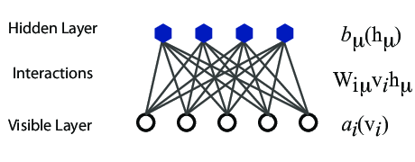
The network
The network layers:- A function \( \mathbf{x} \) that represents the visible layer, a vector of \( M \) elements (nodes). This layer represents both what the RBM might be given as training input, and what we want it to be able to reconstruct. This might for example be the pixels of an image, the spin values of the Ising model, or coefficients representing speech.
- The function \( \mathbf{h} \) represents the hidden, or latent, layer. A vector of \( N \) elements (nodes). Also called "feature detectors".
Joint distribution
The restricted Boltzmann machine is described by a Boltzmann distribution
$$
\begin{align}
P_{rbm}(\mathbf{x},\mathbf{h}) = \frac{1}{Z} e^{-\frac{1}{T_0}E(\mathbf{x},\mathbf{h})},
\tag{5}
\end{align}
$$
where \( Z \) is the normalization constant or partition function, defined as
$$
\begin{align}
Z = \int \int e^{-\frac{1}{T_0}E(\mathbf{x},\mathbf{h})} d\mathbf{x} d\mathbf{h}.
\tag{6}
\end{align}
$$
It is common to ignore \( T_0 \) by setting it to one.
Defining different types of RBMs
There are different variants of RBMs, and the differences lie in the types of visible and hidden units we choose as well as in the implementation of the energy function \( E(\mathbf{x},\mathbf{h}) \).
RBMs were first developed using binary units in both the visible and hidden layer. The corresponding energy function is defined as follows:
$$
\begin{align}
E(\mathbf{x}, \mathbf{h}) = - \sum_i^M x_i a_i- \sum_j^N b_j h_j - \sum_{i,j}^{M,N} x_i w_{ij} h_j,
\tag{7}
\end{align}
$$
where the binary values taken on by the nodes are most commonly 0 and 1.
Another variant is the RBM where the visible units are Gaussian while the hidden units remain binary:
$$
\begin{align}
E(\mathbf{x}, \mathbf{h}) = \sum_i^M \frac{(x_i - a_i)^2}{2\sigma_i^2} - \sum_j^N b_j h_j - \sum_{i,j}^{M,N} \frac{x_i w_{ij} h_j}{\sigma_i^2}.
\tag{8}
\end{align}
$$
Representing the wave function
The wavefunction should be a probability amplitude depending on \( \boldsymbol{x} \). The RBM model is given by the joint distribution of \( \boldsymbol{x} \) and \( \boldsymbol{h} \)
$$
\begin{align}
F_{rbm}(\mathbf{x},\mathbf{h}) = \frac{1}{Z} e^{-\frac{1}{T_0}E(\mathbf{x},\mathbf{h})}.
\tag{9}
\end{align}
$$
To find the marginal distribution of \( \boldsymbol{x} \) we set:
$$
\begin{align}
F_{rbm}(\mathbf{x}) &= \sum_\mathbf{h} F_{rbm}(\mathbf{x}, \mathbf{h})
\tag{10}\\
&= \frac{1}{Z}\sum_\mathbf{h} e^{-E(\mathbf{x}, \mathbf{h})}.
\tag{11}
\end{align}
$$
Now this is what we use to represent the wave function, calling it a neural-network quantum state (NQS)
$$
\begin{align}
\Psi (\mathbf{x}) &= F_{rbm}(\mathbf{x})
\tag{12}\\
&= \frac{1}{Z}\sum_{\boldsymbol{h}} e^{-E(\mathbf{x}, \mathbf{h})}
\tag{13}\\
&= \frac{1}{Z} \sum_{\{h_j\}} e^{-\sum_i^M \frac{(x_i - a_i)^2}{2\sigma^2} + \sum_j^N b_j h_j + \sum_{i,j}^{M,N} \frac{x_i w_{ij} h_j}{\sigma^2}}
\tag{14}\\
&= \frac{1}{Z} e^{-\sum_i^M \frac{(x_i - a_i)^2}{2\sigma^2}} \prod_j^N (1 + e^{b_j + \sum_i^M \frac{x_i w_{ij}}{\sigma^2}}).
\tag{15}\\
\tag{16}
\end{align}
$$
Choose the cost/loss function
Now we don't necessarily have training data (unless we generate it by using some other method). However, what we do have is the variational principle which allows us to obtain the ground state wave function by minimizing the expectation value of the energy of a trial wavefunction (corresponding to the untrained NQS). Similarly to the traditional variational Monte Carlo method then, it is the local energy we wish to minimize. The gradient to use for the stochastic gradient descent procedure is
$$
\begin{align}
\frac{\partial \langle E_L \rangle}{\partial \theta_i}
= 2(\langle E_L \frac{1}{\Psi}\frac{\partial \Psi}{\partial \theta_i} \rangle - \langle E_L \rangle \langle \frac{1}{\Psi}\frac{\partial \Psi}{\partial \theta_i} \rangle ),
\tag{17}
\end{align}
$$
where the local energy is given by
$$
\begin{align}
E_L = \frac{1}{\Psi} \hat{\mathbf{H}} \Psi.
\tag{18}
\end{align}
$$
Electrons in a harmonic oscillator trap in two dimensions
The Hamiltonian of the quantum dot is given by
$$ \hat{H} = \hat{H}_0 + \hat{V},
$$
where \( \hat{H}_0 \) is the many-body HO Hamiltonian, and \( \hat{V} \) is the inter-electron Coulomb interactions. In dimensionless units,
$$ \hat{V}= \sum_{i < j}^N \frac{1}{r_{ij}},
$$
with \( r_{ij}=\sqrt{\mathbf{r}_i^2 - \mathbf{r}_j^2} \).
This leads to the separable Hamiltonian, with the relative motion part given by (\( r_{ij}=r \))
$$
\hat{H}_r=-\nabla^2_r + \frac{1}{4}\omega^2r^2+ \frac{1}{r},
$$
plus a standard Harmonic Oscillator problem for the center-of-mass motion. This system has analytical solutions in two and three dimensions (M. Taut 1993 and 1994).
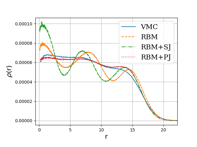
Quantum dots and Boltzmann machines, onebody densities \( N=6 \), \( \hbar\omega=0.1 \) a.u.
Onebody densities \( N=30 \), \( \hbar\omega=1.0 \) a.u.
Onebody densities \( N=30 \), \( \hbar\omega=0.1 \) a.u.
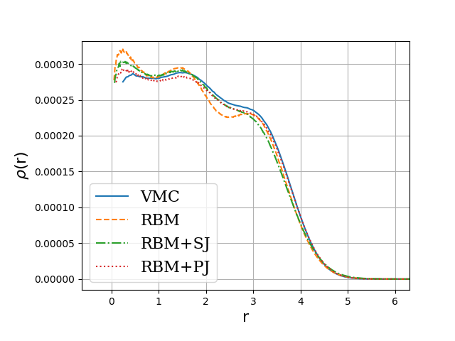
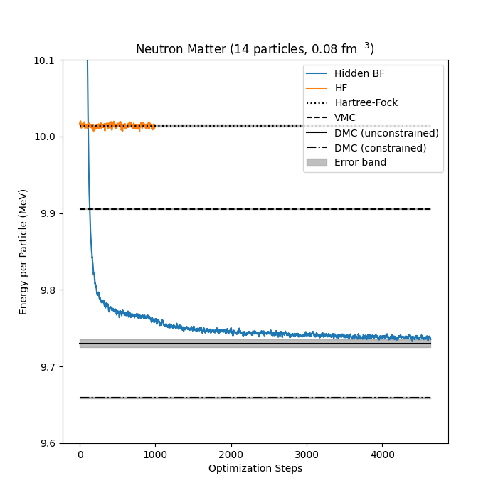
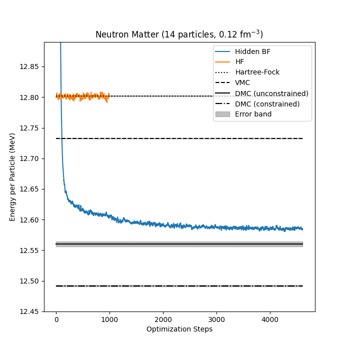
Neutron matter with \( N=14 \) neutron
Jane Kim, Bryce Fore, Alessandro Lovato and MHJ, in preparation

Neutron matter with \( N=14 \) neutron
Jane Kim, Bryce Fore, Alessandro Lovato and MHJ, in preparation
Neutron matter with \( N=14 \) neutron
Jane Kim, Bryce Fore, Alessandro Lovato and MHJ, in preparation
!Split
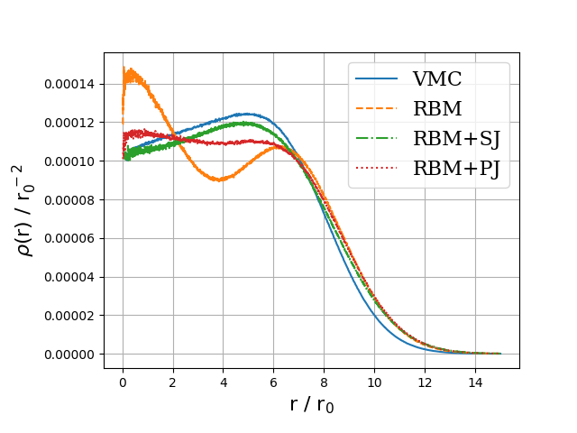
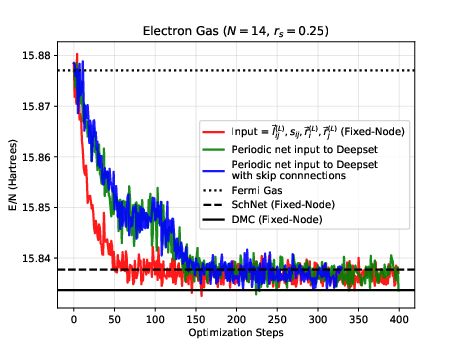
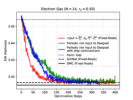
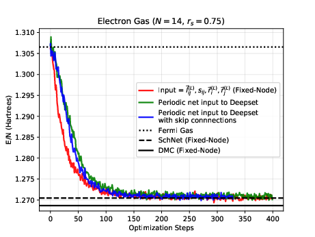
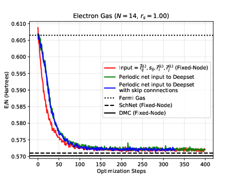
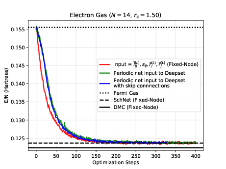
The electron gas in three dimensions with \( N=14 \) electrons (Various Wigner-Seitz Radii)
Jane Kim, Bryce Fore, Alessandro Lovato and MHJ, in preparation and Nordhagen, Kim, Fore, Lovato and MHJ, ArXiv 2210.00365
The electron gas in three dimensions with \( N=14 \) electrons (Various Wigner-Seitz Radii)
Jane Kim, Bryce Fore, Alessandro Lovato and MHJ, in preparation and Nordhagen, Kim, Fore, Lovato and MHJ, ArXiv 2210.00365
The electron gas in three dimensions with \( N=14 \) electrons (Various Wigner-Seitz Radii)
Jane Kim, Bryce Fore, Alessandro Lovato and MHJ, in preparation and Nordhagen, Kim, Fore, Lovato and MHJ, ArXiv 2210.00365
The electron gas in three dimensions with \( N=14 \) electrons (Various Wigner-Seitz Radii)
Jane Kim, Bryce Fore, Alessandro Lovato and MHJ, in preparation and Nordhagen, Kim, Fore, Lovato and MHJ, ArXiv 2210.00365
The electron gas in three dimensions with \( N=14 \) electrons (Various Wigner-Seitz Radii)
Jane Kim, Bryce Fore, Alessandro Lovato and MHJ, in preparation and Nordhagen, Kim, Fore, Lovato and MHJ, ArXiv 2210.00365
The electron gas in three dimensions with \( N=14 \) electrons (Various Wigner-Seitz Radii)
Jane Kim, Bryce Fore, Alessandro Lovato and MHJ, in preparation and Nordhagen, Kim, Fore, Lovato and MHJ, ArXiv 2210.00365
The electron gas in three dimensions with \( N=14 \) electrons (Various Wigner-Seitz Radii)
Jane Kim, Bryce Fore, Alessandro Lovato and MHJ, in preparation and Nordhagen, Kim, Fore, Lovato and MHJ, ArXiv 2210.00365
The electron gas in three dimensions with \( N=14 \) electrons (Various Wigner-Seitz Radii)
Jane Kim, Bryce Fore, Alessandro Lovato and MHJ, in preparation and Nordhagen, Kim, Fore, Lovato and MHJ, ArXiv 2210.00365
Neutron matter with \( N=14 \) neutron
Bryce Fore, Jane Kim, Alessandro Lovato and MHJ, in preparation
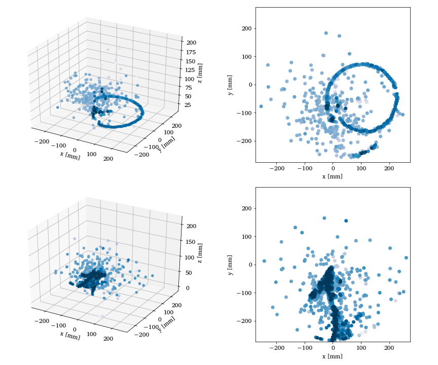
Unsupervised learning in nuclear physics, Argon-46 by Solli, Bazin, Kuchera, MHJ, Strauss.
Two- and three-dimensional representations of two events from the Argon-46 experiment. Each row is one event in two projections, where the color intensity of each point indicates higher charge values recorded by the detector. The bottom row illustrates a carbon event with a large fraction of noise, while the top row shows a proton event almost free of noise.