Quantum Computing and Quantum Mechanics for Many Interacting Particles

What is this talk about?

Why? Basic motivation

Basic activities, Overview

Slides at https://mhjensenseminars.github.io/MachineLearningTalk/doc/pub/quantumcomputing/html/quantumcomputing-reveal.html

Interfacing with Gemini and dScience

During the last two years we have started a large scientific activity on Quantum Computing and Machine Learning at the Center for Computing in Science Education (CCSE), with three PhD students hired since October 2019 (Øyvind Sigmundsson Schøyen, October 2019, Stian Bilek, September 2020, and Jonas Boym Flaten, December 2020) and several master of Science students. This activity spans from the development of quantum-mechanical many-particle theories for studying systems of interest for making quantum computers, via the development of quantum algorithms for solving quantum mechanical problems to exploring quantum machine learning algorithms.

From the fall of 2021 we expect to hire a new PhD student working on quantum computing via the recent EU funded project CompSci, administered by the CCSE. At present we have also four Master of Science students working on the above topics. They would be potential candidates for future PhD fellowships.

Quantum Engineering

Candidate systems

1. Superconducting Josephon junctions
2. Single photons
3. Trapped ions and atoms
4. Nuclear Magnetic Resonance
5. Quantum dots, expt at MSU
6. Point Defects in semiconductors, expt at UiO
7. more

Electrons (quantum dots) on superfluid helium

Electrons on superfluid helium represent a promising platform for investigating strongly-coupled qubits.

Therefore a systematic investigation of the controlled generation of entanglement between two trapped electrons under the influence of coherent microwave driving pulses, taking into account the effects of the Coulomb interaction between electrons, is of significant importance for quantum information processing using trapped electrons.

Quantum algorithms for solving many-body problems, simple model

The pairing model consists of \( 2N \) fermions that occupy \( N \) of \( P \) energy levels. The fermions can only change energy level by pair. It's Hamiltonian is

 
$$ \begin{align} H=\sum_{p\sigma} \delta_pa_{p\sigma}^{\dagger}a_{p\sigma}+\sum_{pq}g_{pq}a_{p+}^{\dagger}a_{p-}^{\dagger}a_{q-}a_{q+} , \tag{1} \end{align} $$

 
where \( p \) and \( q \) sum over the set \( \{1,2,...,P\} \) and \( \sigma \) sums over the set \( \{+,-\} \). Also, \( a \) and \( a^{\dagger} \) are the fermionic creation and annihilation operators.

More on the pairing model

If one assumes that energy levels are never half filled (always occupied by either 0 or 2 fermions), then the pairing model is equivalent to a system of \( N \) pairs of fermions that occupy \( P \) doubly-degenerate energy levels

 
$$ \begin{align} H = 2\sum_{p} \delta_pA_p^{\dagger}A_p+\sum_{pq}g_{pq}A_p^{\dagger}A_q, \tag{2} \end{align} $$

 
where \( p \) and \( q \) sum from over the set \( \{1,...,p\} \) and

 
$$ \begin{align*} A_p &= a_{p-}a_{p+} \\ A^{\dagger}_p &= a^{\dagger}_{p+}a^{\dagger}_{p-}, \end{align*} $$

 
are the fermionic pair creation and annihilation operators.

Unitary Coupled Cluster Ansatz

The unitary coupled cluster ansatz is

 
$$ \begin{align} \vert\Psi\rangle=e^{T-T^{\dagger}}\vert\Phi\rangle, \tag{3} \end{align} $$

 
and

 
$$ \begin{align} \vert\Psi\rangle=\exp{(T_1-T_1^{\dagger})}\vert\Phi\rangle, \tag{4} \end{align} $$

 
where \( \vert\Phi\rangle \) is a Fock state and \( T=\sum_{k=1}^AT_k \).

Technicalities

Since our Hamiltonian only has one body terms. We will truncate to \( T=T_1 \) where

 
$$ \begin{align} T_1=\sum_{ia}t_i^aA_a^{\dagger}A_i. \tag{5} \end{align} $$

 
Thus, we define our ansatz as

 
$$ \begin{align} \vert\Psi(\theta)\rangle=\exp\left\{\sum_{ia}t_i^a\left(A_a^{\dagger}A_i-A_aA_i^{\dagger}\right)\right\}\vert\Phi\rangle. \tag{6} \end{align} $$

 
We define the set of angles \( \theta=\{t_i^a \ | \ i < F, \ a \geq F\} \) where \( F \) is the number of particles below the Fermi level.

Mapping Pair Operators to Pauli Gates

The Jordan-Wigner transformation from pair operators to Pauli matrices is

 
$$ \begin{align} A_p &= \frac{X_p+iY_p}{2} \tag{7}\\ A_p^{\dagger} &= \frac{X_p-iY_p}{2}, \tag{8} \end{align} $$

 
where \( P_i\equiv \left(\bigotimes_{n=1}^{i-1}I\right)\otimes P\otimes\left(\bigotimes_{n=i+1}^NI\right) \) where \( P \in \{X,Y,Z\} \) and \( N \) is the total number of particles.

Mapping the Ansatz

Applying this transformation

 
$$ \begin{align} A_a^{\dagger}A_i-A_aA_i^{\dagger} &=\left(\frac{X_a-iY_i}{2}\right)\left(\frac{X_a+iY_i}{2}\right) \tag{9}\\ &-\left(\frac{X_a+iY_i}{2}\right)\left(\frac{X_a-iY_i}{2}\right) \tag{10}\\ &=\frac{i}{2}\left(X_aY_i-Y_aX_i\right), \tag{11} \end{align} $$

The ansatz becomes

 
$$ \begin{align} \vert\Psi(\theta)\rangle =\exp\left\{\frac{i}{2}\sum_{ia}t_i^a\left(X_aY_i-Y_aX_i\right)\right\}\vert\Phi\rangle. \tag{12} \end{align} $$

Trotter approximation

 
$$ \begin{align} \tag{13} \vert\Psi(\theta)\rangle &\approx\prod_{ia}\exp\left\{\frac{i}{2}t_i^a\left(X_aY_i-Y_aX_i\right)\right\}\vert\Phi\rangle \\ &\equiv \prod_{ia}A_{ia}\vert\Phi\rangle. \tag{14} \end{align} $$

Mapping the Hamiltonian

First, we rewrite the Hamiltonian

 
$$ \begin{align} H &=2\sum_{p}\delta_pa_p^{\dagger}a_p+\sum_{pq}g_{pq}a_p^{\dagger}a_q \tag{15}\\ &=\sum_{p}\left(2\delta_p+g_{pq}\right)a_p^{\dagger}a_p+\sum_{p\neq q}g_{pq}a_p^{\dagger}a_q. \tag{16} \end{align} $$

 
Applying the transformation to the first term in the Hamiltonian

 
$$ \begin{align} a^{\dagger}_pa_p=\left(\frac{X_p-iY_p}{2}\right)\left(\frac{X_p+iY_p}{2}\right)=\frac{I_p-Z_p}{2}. \tag{17} \end{align} $$

More manipulations

 
$$ \begin{align} \sum_{p\neq q}a_p^{\dagger}a_q =\sum_{p < q}a_p^{\dagger}a_q+\sum_{q < p}a_p^{\dagger}a_q =\sum_{p < q}a_p^{\dagger}a_q+a_pa_q^{\dagger}, \tag{18} \end{align} $$

 
which we arrive at by swapping the indices \( p \) and \( q \) in the second sum and combining the sums. Applying the transformation

 
$$ \begin{align} a_p^{\dagger}a_q+a_pa_q^{\dagger} &=\left(\frac{X_p-iY_p}{2}\right)\left(\frac{X_q+iY_q}{2}\right) \tag{19}\\ &+\left(\frac{X_p+iY_p}{2}\right)\left(\frac{X_q-iY_q}{2}\right) \tag{20}\\ &=\frac{1}{2}\left(X_pX_q+Y_pY_q\right). \tag{21} \end{align} $$

Hamiltonian

 
$$ \begin{align*} H = \sum_p\left(2\delta_p+g_{pq}\right)\left(\frac{I_p-Z_p}{2}\right) +\sum_{p < q}g_{pq}\frac{X_pX_q+Y_pY_q}{2} \end{align*} $$

Exact and Calculated Correlation Energies vs Pairing Strength for \( (p,n)=(4,2) \)

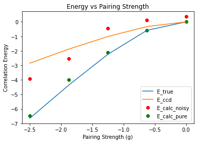
Note: \( p \) is the number of doubly-degenerate levels and \( n \) is the number of pairs of fermions.

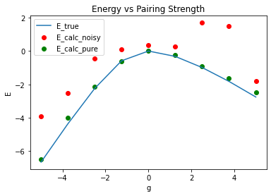
Exact and Calculated Correlation Energies vs Pairing Strength for \( (p,n)=(5,2) \)

Quantum Machine Learning

The emergence of quantum computers has opened up even more possibilities within the field of machine learning. Since quantum mechanics is known to create patterns which are not believed to be efficiently produced by classical computers, it is natural to hypothesize that quantum computers may be able to outperform classical computers on certain machine learning tasks. There are several interesting approaches to machine learning from a quantum computing perspective - from running existing algorithms or parts of these more efficiently, to exploring completely new algorithms that are specifically developed for quantum computers. Recent results show that quantum neural networks are able to achieve a significantly better effective dimension than comparable classical neural networks.

More on Quantum Machine Learning

A few examples of existing algorithms that exhibit a speed up on quantum computers are \( k \)-nearest neighbors, support vector machines and \( k \)-means clustering.

Among algorithmic approaches that are specifically designed for quantum computers we find so-called parameterized quantum circuits. These are hybrid quantum-classical methods where the input-output relation is being produced by a quantum computer, while a classical computer is responsible for updating the model parameters during training.

Present Plans

1. Quantum circuit optimization
2. Quantum Boltzmann Machines

So-called Boltzmann Machines (BMs) define a machine learning method that aims to model probability distributions and has played a central role in the development of deep learning methods.

It has since been shown that BMs are universal approximators of discrete probability distributions, meaning that they can approximate any discrete distribution arbitrarily well. Our research group has lately conducted several investigations of BMs applied to quantum-mechanical problems, with several interesting results.

Conclusions and where do we stand

Lots of interesting research directions.

1. We have used many-body methods like time-dependent full configuration interaction theory to design quantum circuits, in close collaboration with experimentalists
2. Successfully applied various quantum algorithms to many-body systems
3. Quantum machine learning, just started
4. What could be of interest to the Gemini center?